Commodity price fluctuations and the EROI of oil – how the availability of surplus energy affects non-fuel commodity prices
Abstract
We study the long-term effect of a changing energy return on investment (EROI) of oil on non- fuel commodity prices. Compared to economic growth, interest rates and uncertainty, the EROI of oil is the main driver of commodity price variations since 1938. A change in the EROI of oil accounts for up to 30% of the variation in commodity prices. We show that over the past 100 years, periods of low EROI have been correlated with higher commodity prices and vice versa. Commodity prices thus depend on the amount of surplus energy available for society. As renewables show substantially lower EROI values than fossil fuels used decades ago, the energy transition poses major challenges not only to our society but also to resource-intensive companies. The adoption of new business practices like the circular economy fosters the development of strategies increasing the EROI and reducing the large demand for external sources of energy and raw materials.
1 Introduction
Everything that happens in the world uses energy of one kind or another. Historically, the pre-agrarian hunter-gather era was characterized by an approximate energy balance where the energy each person derived from his food was almost the same which he expanded in finding that food. When humans started domesticating plants and animals more than 10,000 years ago, the agriculture revolution led to a liberation of surplus energy and the development of early societies. During that era, investment began when the energy surplus was deployed into the creation of capital goods instead of immediate consumption letting evolve simple shipping and trading industries (Morgan, 2013). The exploitation of fossil fuels during the industrial revolution vastly multiplied not only the energy availability but also the per capita use of energy. Due to the discovery of the heat engine it only took a little energy input to get a lot of energy out of fossil fuels, lifting ordinary citizens out of poverty into a developing middle class (Buchanan, 2019). Today, energy plays a major role throughout social and economic development and remains central to all politics.
However, it requires energy to produce energy. As the exploitation of any resource requires effort, to find it, gather it and process it into useful forms, it is not just the energy produced what matters most, but the relation between the energy that is produced and the amount of energy that is needed in the production process. The key technical term describing the ratio of energy returned to energy invested is called Energy Return On Investment (EROI):
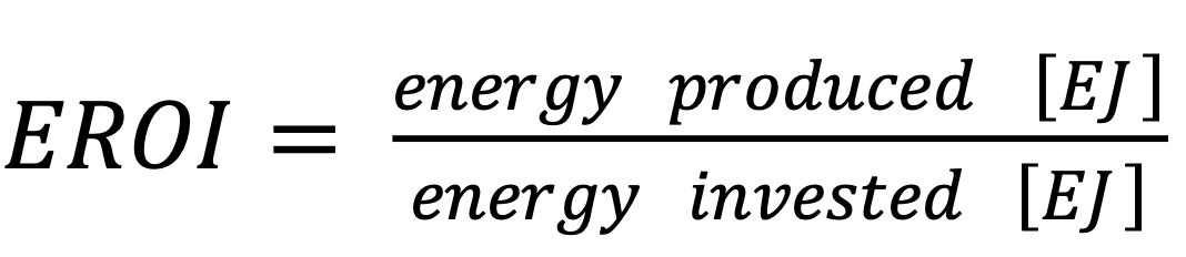
As a dimensionless quantity, EROI reflects the energy density and ease of access of the corresponding source of energy (Buchanan, 2019). A large/small EROI indicates that the energy from that source is easy/difficult to get. For an EROI equal to 1, there is no energy return on the energy invested. The investment would be wasted.
Since the middle of the last century the extraction of fossil fuels is getting more complex and an increasing proportion of the energy output is diverted to producing that energy (Lambert et al. 2012). Accordingly, global EROI figures for our most important fuels (except coal) have been declining for some time. Global oil and gas production went from ratios of over 80 or 90:1 in the 1930s to 35:1 in the 1990s and 18:1 in the 2000s (Lambert, et al., 2013). Especially tar sands in Canada show small EROI values of maximum 11:1 (Lambert, et al., 2013). This trend is not likely to reverse as renewables and other non-renewables show substantially lower EROI values than fossil fuels used decades ago (Buchanan, 2019). Nuclear power has EROI values of around 5:1 to 15:1, averaged over the entire fuel cycle (Lenzen, (2018), Lambert, et al., (2013)), wind power shows values of around 18:1 (Lambert, et al., 2013)) and hydropower can have a very high EROI for some installations, but can also be quite low. In a meta-analysis of 232 references Bhandari, et al. (2015) show that EROI values for mono- and poly-crystalline silicon PV modules vary between 6 and 16:1. Other renewables like US corn ethanol are estimated to have an EROI of less than 2:1 (Lambert, et al., 2013). However, the consequences of the energy transition to a more sustainable future and lower EROI values on economic conditions and especially on commodity price developments are unclear (Court & Fizaine 2017).
Furthermore, the oil price boom between 2005 and 2008 and the subsequent market collapse, causes serious concerns among economists as to whether today’s energy prices may be sufficient to guide decisions about the energy future (Hall et al. 2009). As proposed in Hall et al. (2009), the analysis of EROI values might provide an alternative view for assessing advantages and disadvantages of various energy sources. Hence, considerations of EROI values provide valuable information on future, fundamental market developments which market prices could not account for, cf. Hall et al. (2009) and Hamilton (2012).
Like all forms of economic output, also the extraction and processing of raw commodities largely depends on the amount of surplus energy available to the system. Hence, in our paper we estimate the effect of the decreasing EROI of oil on long-term commodity price developments between 1900 and 2014. Relying on the price-based EROI of Court & Fizaine (2017), we extend existing literature on long-term commodity assessments like Byrne et al. (2013) to gain a better understanding of long-run movements in commodity prices.
To the best of our knowledge, we are the first who examine the long-run effect of declining EROI of oil on an index of non-energy commodity prices. We find evidence that commodity prices depend on the amount of surplus energy available to economies. Since 1938, we show that EROI is the most influential variable and explains up to 30% of commodity price fluctuations (Chapter 4). The lower the EROI, the higher are commodity prices. During times of weak economic growth, the EROI effect on commodity prices is stronger than in times of strong economic growth. We thus conclude that simultaneously considering GDP growth rates and EROI values of most important energy sources helps to estimate fundamental effects the change in main energy sources might have on commodity price developments.
In the remainder of this paper, we continue with a literature review, followed by an overview of the data used in the model and the determination of the EROI of oil. The penultimate section determines the driving factors of commodity price developments in a structural VAR approach and highlights most important learnings of our approach while the final section concludes.
2 Literature review
Historically, commodity prices are driven by various factors and determined by long-term trends, long cycles, and short-run fluctuations (Arezki et al. 2014). A large body of literature has been developed based on the Prebisch (1950) and Singer (1950) (PS) thesis focusing on long-run commodity price trends. Authors argue that over the long run, prices of primary commodities exhibit declining trends relative to prices of manufactured goods. These findings could be explained by low-income elasticities of demand for commodities or technological and productivity differentials between industrial and non-industrial countries (Harvey et al. 2017). An excellent overview of most important papers in the field of trend analysis of long-run commodity price series is given in Baffes & Etienne (2016).
Analyzing long cycles, the literature finds strong empirical evidence that global economic growth is one of the key drivers of commodity demand (Bruno et al. 2016). Barsky & Kilian (2001) show that commodity prices are influenced by macroeconomic conditions. Especially in the early 1970s, they argue that industrial commodity price increases were consistent with an economic boom driven by monetary expansion. Similarly, Carter et al. (2011) focus on two major commodity booms and busts episodes in 1974 and 2008. As the primary reason behind this development they find contemporaneous supply and demand shocks coinciding with low inventory levels and macroeconomic shocks. Jeffrey A. Frankel (2006) examines connections between monetary policy, agriculture and mineral commodities and claims that low real interest rates lead to high real commodity prices. Based on a structural VAR model, Akram (2009) confirms that commodity prices significantly increase in response to reductions in real interest rates and a weaker US dollar. Lombardi et al. (2012) find exchange rates and economic activity to be important drivers for individual non-energy commodity prices between the 1970s and 2008.
Apart from the aforementioned key drivers of commodity prices another branch of literature focuses on the relation between energy and non-energy commodities. Between 1960 and 2005 Baffes (2007) examines the effect of crude oil prices on the prices of 35 internationally traded primary commodities. Baffes (2007) argues that oil prices affect the supply side of commodities due to fertilizer prices, transportation, or any kind of energy intensive production. Additionally, Baffes & Etienne (2016) and Baffes & Haniotis (2016) find a strong pass-through of crude oil price changes to an overall non-energy commodity index. The latter also show that real income negatively affects real agriculture prices in the long run, whereas energy costs, monetary conditions and inventories are rather short-term prices drivers. Similarly, Nazlioglu et al. (2013) suggest dynamic interrelationships between energy and agriculture markets. In contrast, Alghalith (2010) and Chang & Su (2010), and Lombardi et al. (2012) do not find direct price relations between fuel and agriculture commodity prices.
We extend the current literature by adopting the concept of energy return on investment (EROI) and its implications on commodity prices. As economic systems heavily rely on available energy, Stern (2011) assumes that when energy is scarce it might impose strong constraints on economic growth. In addition, as energy is a key input variable for the extraction and production of raw commodities, it is of great interest how changing energy availability affects the supply side of commodity prices. The economic literature on the concept of EROI and its implications for economic growth has emerged in recent years only. For a good review of the literature see Murphy (2014). He concludes that the EROI of global oil production is declining and that the relation between EROI and the price of oil is inverse and exponential. Murphy (2014) thus proposes, that declining EROI impedes long-term economic growth and will come at higher financial, energetic and environmental costs. Similar conclusions can be found in Murphy & Hall (2011) and Fizaine & Court (2016). Hall et al. (2014) give a detailed description of different types of EROI analysis and its boundaries. Court & Fizaine (2017) follow up on this analysis and introduce a price based methodology to estimate long-term global EROI of coal, oil, and gas (from 1800 to 2012). Their results are consistent with already existing estimations of global oil and gas production as in Gagnon et al. (2009) and theoretical models developed in Dale et al. (2012). Court & Fizaine (2017) conclude that the EROI of global oil productions reached its maximum value of 80:1 in the 1930s-40s and has declined subsequently. An EROI of 80:1 indicates that 80 units of energy output require one unit of energy input to produce that energy.
Combining various approaches discussed in the literature, we estimate how a decreasing EROI of oil affects commodity price developments in the following sections.
3 Data description and the measurement of EROI
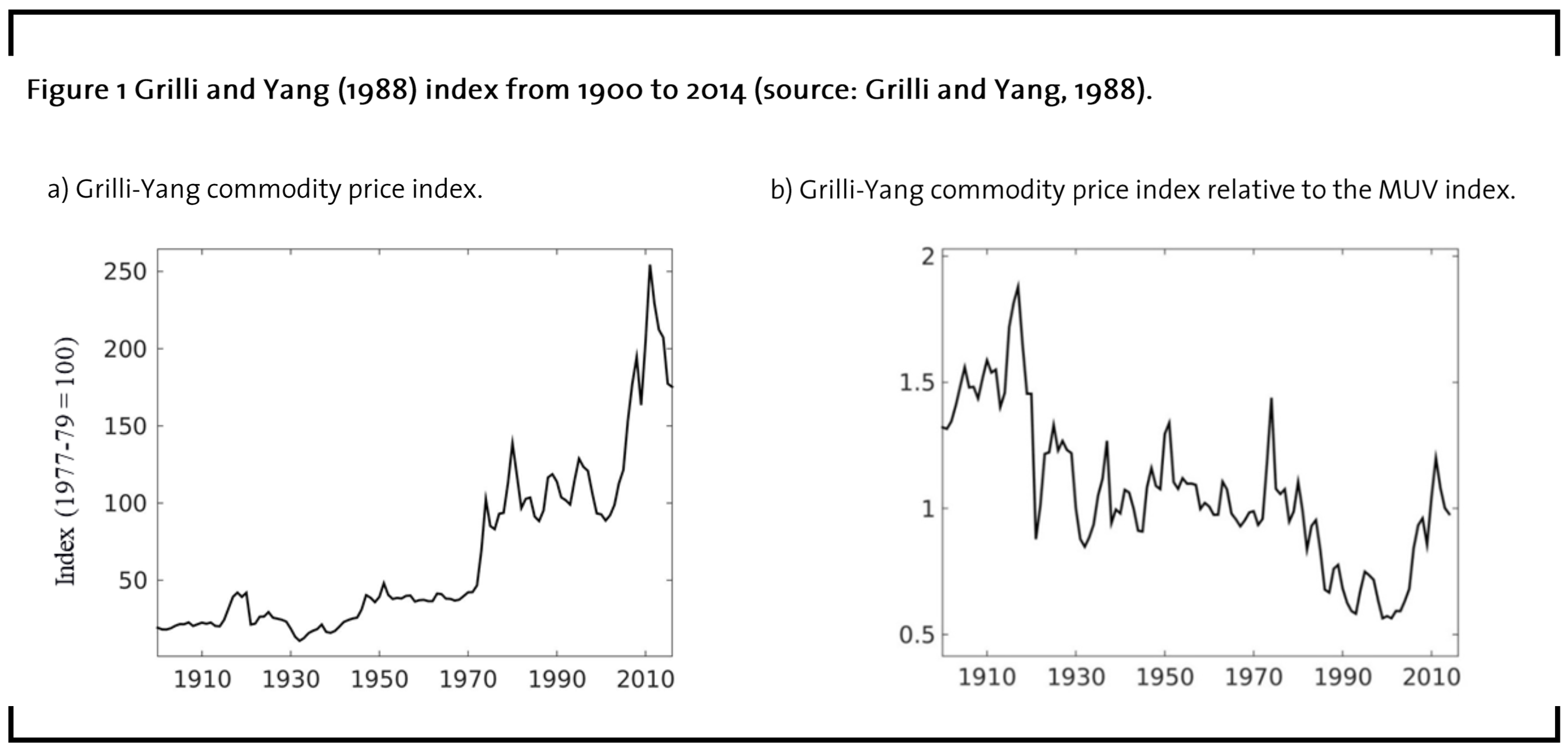
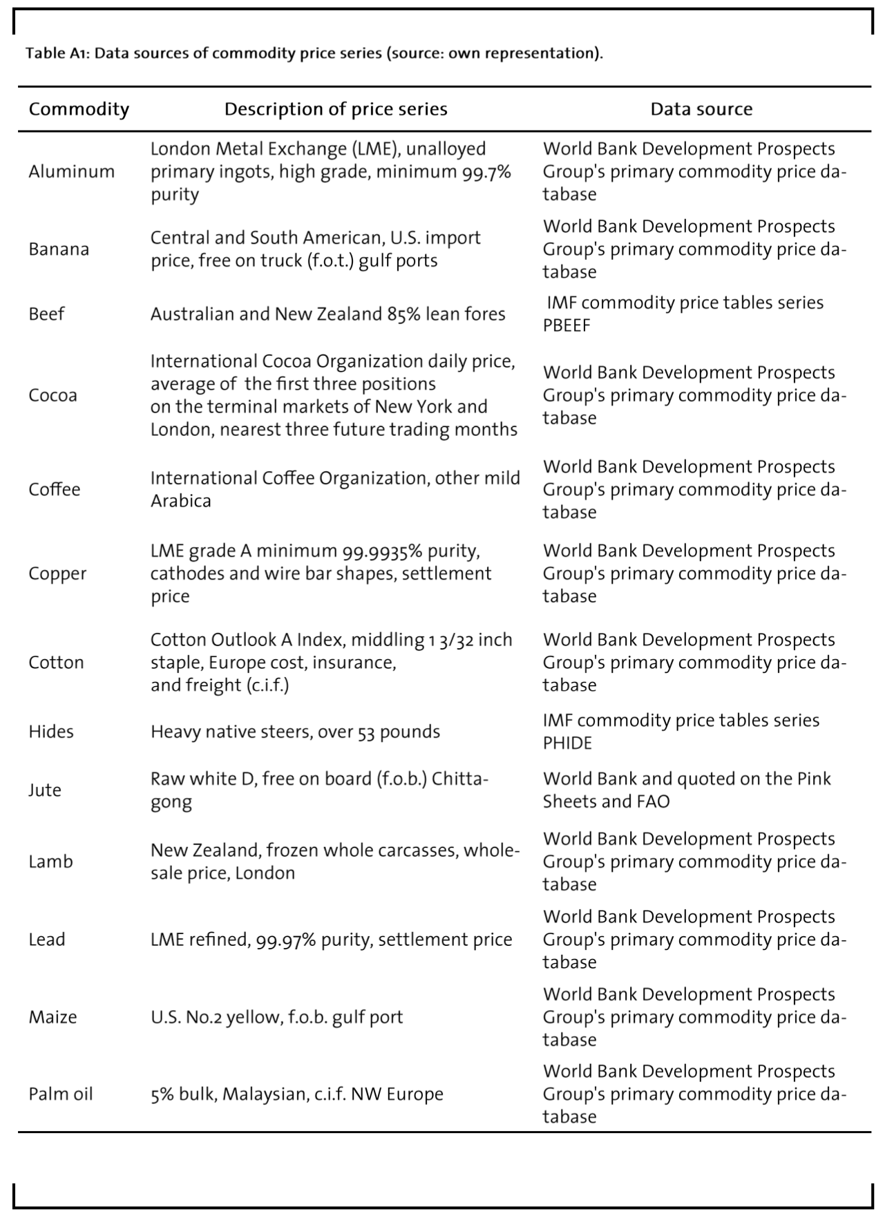
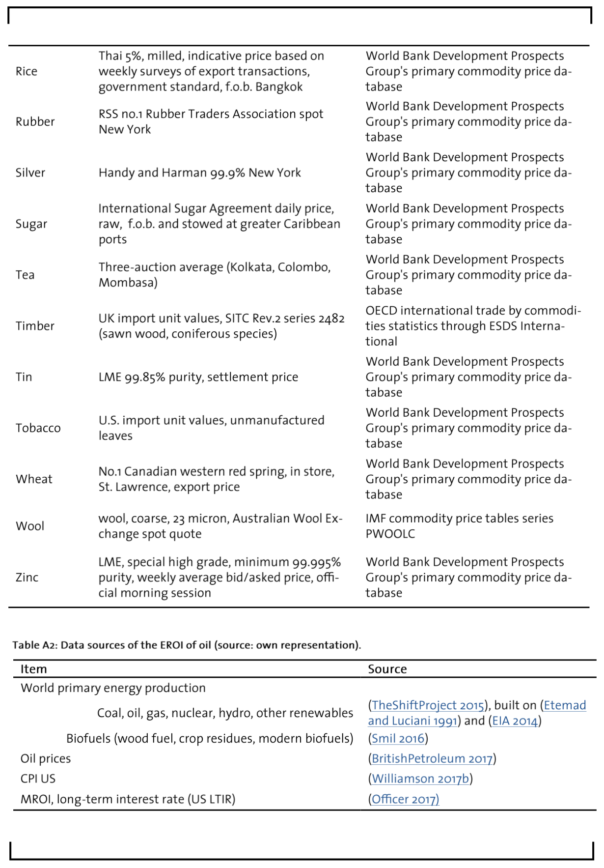
We rely on the widely used Grilli & Yang (1988) commodity price index (GYCPI) to assess long-term effects of decreasing surplus energy on commodity prices. For the period 1900 to 1986 the trade-weighted index is composed of 24 primary non-fuel commodity prices deflated by the manufacturing unit value index (MUV). The MUV is one of the most frequently used deflator in the literature and is determined as a trade-weighted index of exports of manufactured commodities from France, Germany, Japan, United Kingdom, and United States to developing countries (Pfaffenzeller et al. 2007). We have updated the GYCPI based on commodity price series suggested in Pfaffenzeller et al. (2007) to 2014. Descriptive statistics of the individual commodity return series are shown in Table 1 and the detailed summary of commodities used in our study can be found in Table A1.
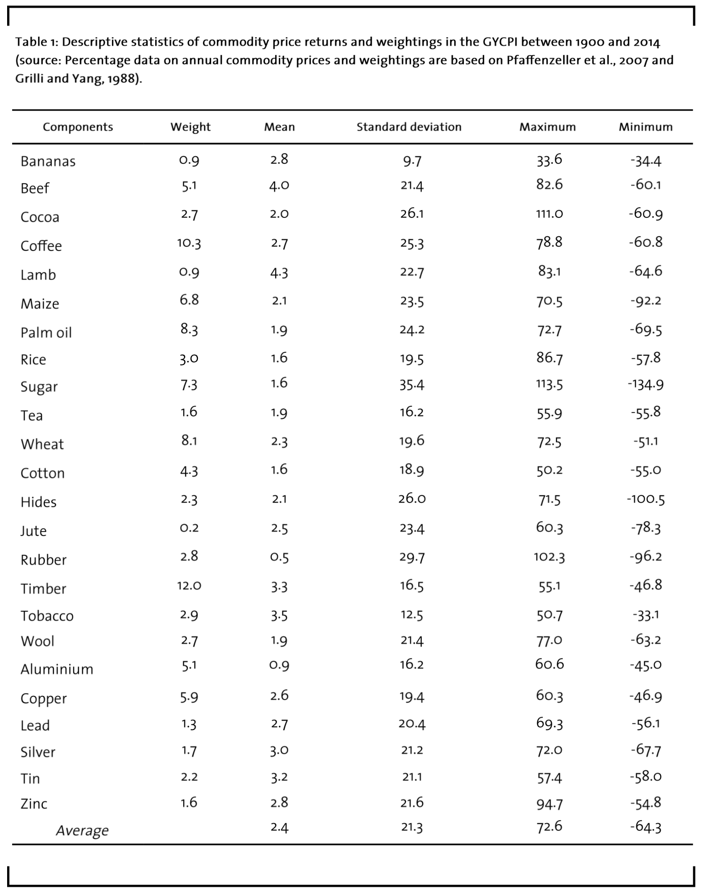
Figure 1 shows the GYCPI and the GYCPI relative to the MUV index. The GYCPI shows an upward trend over time whereas real commodity prices decline (GYCPI relative to MUV) until the beginning of the 2000s. Both indices exhibit sideways movements between the 1950’s and the 1960’s and show a commodity price boom during the 1970’s. Since the early 2000’s we seean increasing trend corresponding to the second global boom in commodity markets, cf. Carter et al. (2011). In the following analysis we rely on the GYCPI relative to MUV.
Which factors drive commodity prices?
Empirical evidence suggests that commodity prices are influenced by macroeconomic conditions, geopolitical uncertainty, and monetary policy (Barsky & Kilian (2001), Jeffrey A. Frankel (2006), Bruno et al. (2016)). First, to approximate global uncertainty, we rely on stock market risk calculated as annualized standard deviations of daily Dow Jones index data (Williamson (2017a)). For a similar approach see Byrne et al. (2013) and references therein.
Second, to estimate how monetary policy affects commodity prices we rely on real US interest rates. As a proxy variable we use short-term interest rates from Officer (2017). Until 1930 they consist of ordinary funds rates from the Federal Reserve and from 1931 to present, they are in the form of 3-months US treasury bills. Intuitively, rising interest rates lead to an increase of investments in fixed income securities as they get more interesting than risky products like commodities. This reduces the demand for commodities and leads to falling commodity prices.
Third, most important drivers of long-term commodity price developments are supply and demand. As already noted in Bruno et al. (2016), there is overwhelming empirical evidence that global economic growth is a key driver of commodity demand (Alquist & Coibion (2014), Kilian (2009)). We use world GDP growth rates as approximation of global demand effects and obtain the data from Maddison (2013) and World Bank. Similar to Byrne et al. (2013), we estimate missing data for world GDP between 1900 and 1950 by linearly interpolating the GDP series of China, USA, India, 12 Western European countries, Latin America, Australia, New Zealand, Canada, and Japan. On the supply side, we focus on the importance of energy availability. The availability of energy is the most important input factor for non-fuel commodities due to fertilizer prices, transportation, or any kind of energy intensive production (Baffes 2007). Motivated by Hall et al. (2009) we rely on the EROI of oil to estimate how changing energy availability affects non-fuel commodity prices. Our analysis is particularly important as the EROI of conventional fossil fuels is decreasing and the EROI of most renewable and non-conventional energy alternatives is substantially lower than the EROI of conventional fossil fuels (Hall et al. 2014).
Determination of the EROI
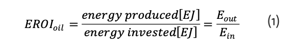
The EROI of oil is measured as the energy output Eout divided by the energy input Ein.
The higher the EROI, the greater is the amount of surplus energy accessible to society (Hall et al. 2014). Until today, there is no single accepted procedure how to estimate EROI for different sources of energy. In order to estimate long-term EROI of oil we thus follow Court & Fizaine (2017) and King & Hall (2011) and use a price based methodology. The EROI based on Court & Fizaine (2017) represents the ratio of annual gross energy produced to annual energy invested.
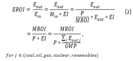
The output or production boundary of the EROI is at the well-head and is estimated based on historical oil production data. The input side covers direct energy expenditures, indirect energy expenditures from physical capital investments, and direct energy embodied in what workers purchase with their payback. Hence, most important variables for the energy input side are oil prices, the global primary energy mix, monetary-return-on-investment (MROI) of the energy sector and energy intensity of capital expenditures in the primary fossil energy sector. The final estimation of the global EROI of oil is as follows1:
1We do not consider storage costs explicitly as data is not available for the period considered in this paper. However, parts of these costs might be related to energy usage and thus partly covered in our EROI-factor.
- Energy Ein invested in global oil system corresponds to the quantity of money Min invested in the sector multiplied by the average energy intensity EI of capital and services installed and used.
- For Min only few data exist. Min is estimated as the quantity of energy produced Eout by the oil sector multiplied by a proxy for annual (not levelized) production costs of oil.
- The production costs of oil are estimated as the unitary price P of oil divided by the monetary-return-on-investment (MROI) of the oil sector. According to Court & Fizaine (2017) and Damodaran (2015), the US fossil energy sector’s MROI is roughly following US long-term interest rates with a 10% risk premium.
- Further assumption: The energy intensity EI is the same for all energy sectors and corresponds to the average energy intensity of the global economy. EI is estimated as the sum of the entire energy output from coal, oil, gas, nuclear, and renewables divided by the gross world product GWP.
- The global EROI for oil reads as follows2:
2All US $ values are expressed in the international Geary-Khamis $1990.
A description of the data sources used in our study is shown in Table A2. For a more detailed view on data and estimation procedure, the interested reader should have a look at Court & Fizaine (2017). Figure 2 shows the annual price-based global EROI of oil from 1900 to 2014 compared with the GYCPI deflated by MUV. It is clear to see, that both series develop in opposite directions. Periods of high EROI values coincide with periods of low real commodity prices and vice versa.
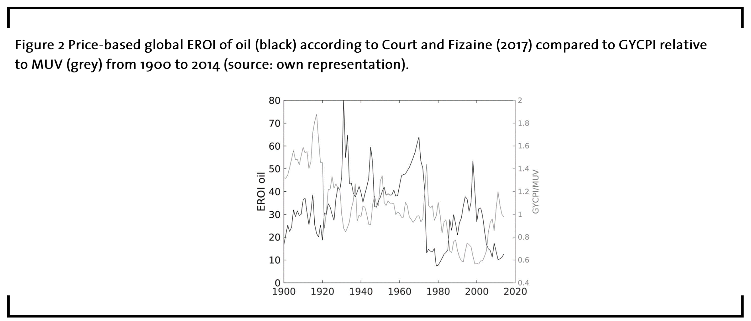
As resources become scarce or technology makes new sources available, the EROI of any energy source may change over time (Buchanan, 2019). Hence, the EROI of oil fluctuates greatly during the past 120 years. The period from 1900 to 1937 was characterized by intensive use of coal and traditional biomass energy. Oil production was only about to start growing but increased rapidly since the late 1930s. EROI levels for oil reached its all-time high in 1931.
During the period from 1938 to 1976 the production of oil surged. Coal and oil were used for the production and use of war machinery. After WWII, the importance of global manufacturing and transportation increased and oil became even more important (Hall et al. 2014). The EROI of oil reached its highest average level during this period and its second peak in 1970. US oil production peaked in the same year. From this year on, OPEC oil has gained increasing importance for world supply. Hence, the EROI of oil decreased and oil prices rose subsequently reflecting the increased amount of energy needed to acquire this fuel, cf. Hall et al. (2014) and Hall & Klitgaard (2012).
In the beginning of the period from 1977to 2014 the Iranian revolution (1978/79) and Iran-Iraq war (beginning of 1980) caused high oil prices and the oil price shock in 1979. Oil extractions which were uneconomic before became economic during this period, leading to lower EROI values, cf. Guilford et al. (2011) and Hall et al. (2014). The following years between mid-80s and early 90s can be described as a period of abundant oil and falling prices which resulted in less oil explorations. Since the oil price peak in 2008 the introduction of new drilling techniques again rapidly increased the oil production in the US. However, over the past two decades the EROI of oil is decreasing as also shown in Murphy & Hall (2011) and Tverberg (2012).
In the following section we investigate to what extend the changing level of EROI affects an index of non-fuel commodity prices.
4 Model description and results
Based on yearly data for 𝒀𝒕 = (∆EROIt, Riskt, ∆GDPt, IRt, ∆GYCPIt) we examine the effect of changing net energy availability on commodity prices within a structural VAR approach. Within this model, EROIt is the log energy returned on investment for oil, Riskt measures the risk of geopolitical and monetary uncertainty as annualized standard deviations of daily Dow Jones index data, GDPt corresponds to log world GDP. Until 1930, IRt are the real US interest rates based on ordinary funds rates from the Federal Reserve and from 1931 to present IRt are 3- months treasury bills of the US. GYCPIt is the log of the Grilli-Yang commodity price index deflated by MUV. To ensure stationary time series we apply the fist-order difference operator Δ. We define the structural VAR approach with p lags as follows
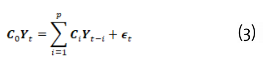
𝝐𝑡 is the vector of serially and mutually uncorrelated structural shocks and we determine the lag length p according to the Schwarz (1978) information criterion. The matrix 𝑪0−1 given in Equation 3 has a recursive structure with reduced-form errors 𝒖𝑡 which are obtained from 𝒖𝒕 = 𝑪0−1 𝝐𝑡:
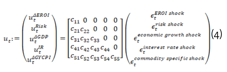
As we rely on the orthogonalization of our VAR system based on a Cholesky decomposition of the reduced-form error’s covariance matrix, our structural system is contemporaneously recursive3. The set-up of the variables is based on the following assumptions:
3A similar model setup can be found in Kilian (2009), Wang et al. (2014), and Lübbers and Posch (2017).
- Economic growth and commodity prices are strongly driven by energy input. As the energy which is used in the extraction process is not available for generating economic output, lower EROI values can have strong influence on economic activity (Buchanan, 2019). Hence, a shock in the EROI of oil will not only have implications on GDP growth rates but also on commodity prices. In addition, changing EROI of oil might simultaneously affect global economic uncertainty and risk in financial markets due to changing energy prices.
- Risk and uncertainty simultaneously affect economic growth, monetary policies and commodity prices as argued in Frankel (2006).
- There is overwhelming empirical evidence that global economic growth is a key driver of commodity demand, as noted in Bruno et al. (2016). A shock in world GDP growth rates thus changes global demands for raw commodities and thereby its prices.
- Monetary policies are adapted to changes in economic conditions. As suggested in Frankel (2006) and Akram (2009), changes in interest rates simultaneously affect commodity prices. Rising interest rates might reduce the demand for commodities and lead to falling commodity prices.
- Finally, commodity prices are simultaneously affected by all other variables.
How do commodity prices react to shocks in EROI and GDP growth rates?
We start by estimating the structural VAR for 𝒀𝒕 = (∆EROIt, Riskt, ∆GDPt, IRt, ∆GYCPIt) to evaluate the effect of varying EROI levels over time and for various sample periods. As we focus on supply and demand shocks, Figure 3 shows the responses of the GYCPI to shocks in the EROI of oil and world GDP growth rates. The 95% confidence bands are estimated from 1000 Monte Carlo simulations. The impulse responses of the GYCPI to real interest rates and uncertainty shocks are shown in Figure A3.
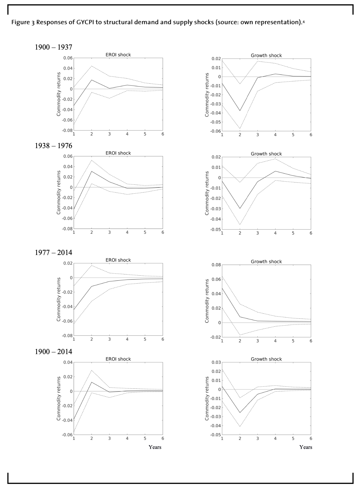 4The graphs show the response of the Grilli-Yang index to a generalized one standard deviation innovation in the EROI of oil and world economic growth for different periods of time. The 95% confidence bands are based on 1000 Monte Carlo simulations.
The period between 1900 and 1937 can be characterized by intensive use of coal and traditional biomass energy rather than oil. Hence, oil’s EROI shocks on GYCPI do not show significant effects on commodity returns. A shock in economic growth rates significantly affects the GYCPI for a short period of time and after two years only. Possibly, this might be explained by volatile economic conditions and WWI.
The following years from 1938 to 1976 can be described as a period of cheap and abundant fossil energy. The total energy consumption per person has more than doubled (Figure 4) and the average level of the EROI of oil reached its highest values (Figure 2). A shock in the EROI of oil thus negatively (contrarily) affects the GYCPI. Intuitively, rising EROI values lead to more surplus energy and decreasing energy costs. This in turn results in lower commodity prices. However, commodity prices seem to overreact on EROI shocks as its effect becomes significantly positive after two years and insignificant subsequently. Shocks in economic growth only show little to no significant effects on the GYCPI.
The most striking results of Figure 3 are the distinct negative responses of commodity prices to shocks in oil EROI values during the last period from 1977 to 2014. This period is characterized by strong economic growth (Figure 4) but lower average EROI values (Figure 2). We conclude, that also decreasing EROI values have a distinct and significant effect on commodity prices. Intuitively, the lower the EROI the less surplus energy is available and the more expansive are commodity prices.
In contrast, the effect of world GDP growth rates shocks on GYCPI is significantly positive. However, the impact of EROI and GDP on GYCPI appears to be of the same size. The time to recover from a shock in EROI and GDP growth rates is approximately 6 months. Over the entire period (1900 to 2014) shocks in the EROI of oil are more important for commodity price movements than shocks in GDP growth rates. Hence, changes on the supply side seem to be more relevant for commodity price movements than those on the demand side.
What is the explanatory ability of our main drivers’ shocks on commodity prices?
In order to examine the amount of information each variable contributes to the other variables in our VAR model, Table 2 summarizes the results of our Forecast Error Variance Decomposition (FEVD) at forecast horizons of one and five years. Between 1900 and 1937 real interest rate shocks account for more than half of the variation in commodity prices. This confirms the findings of Jeffrey A. Frankel (2006) who claims that low real interest rates lead to high real commodity prices, cf. Figure A3. EROI, risk, and GDP growth are less important for commodity prices within that time period. However, demand shocks and supply shocks both almost account for 10% of commodity price variationsover the five-year forecast horizon. During the second period (1938 to 1976), the most important variables are EROI (30.7%), risk (11%), and GDP growth rates (10.3%) which account for 52% of the variations in commodity prices. The importance of these variables reflects macroeconomic and political developments during these years. After WWII strong economic growth, increased manufacturing and transportation drove demand for fossil energy products (Hall et al. 2014) and raw commodities.
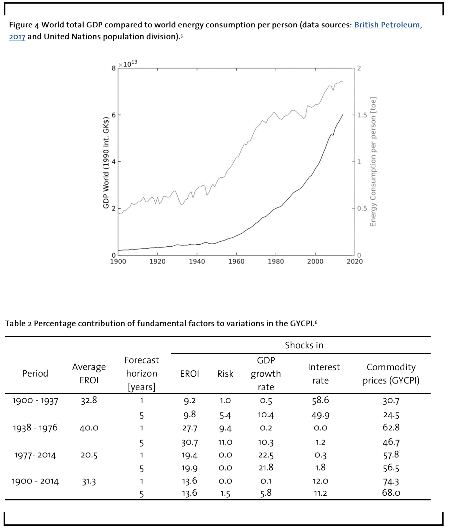
5The world total GDP (black) values are expressed in the international Geary-Khamis 1990$ and energy consumption is given in tons of oil equivalent (toe) per person (grey).
6Thus table compares the percentage contribution of different shocks to the Grilli-Yang index for various time periods and forecast horizons of one and five years.
From 1977 to 2014 economic growth has surged (Figure 4). Our FEVD analysis reveals that GDP growth rates account for more variation in real commodity price changes (22.5%) than shocks in the energy availability (19.4%). Together, shocks in EROI and GDP growth rates almost account for more than 40% of the variation in commodity prices. Interest rates and uncertainty of financial markets only play minor roles. Interestingly, the low impact of financial risk on commodity price fluctuations also suggests that financial markets are not important for long-run commodity price fluctuations. These findings are in line with parts of the literature examining the effect of financial speculation on commodity prices. While the correlation between commodity and equity returns surged during the financial crisis in 2008, Bruno et al. (2016) could not find a significant long-run correlation between those two markets.
Over the entire period (1900 to 2014) and in line with Frankel (2006) we find that real interest rates play a dominant role for the fluctuation of commodity prices. However, its effect was strongest during the beginning of the 20th century and became less important over the years. In accordance with Barsky & Kilian (2001) who argue that industrial commodity price increases in early 1970s were consistent with an economic boom driven by monetary expansion, our results show GDP growth rates to be important for commodity price variations only since the early 1970s. As EROI is the most influential variable for commodity price variations since 1938 explaining more than 19% of commodity price fluctuations, our results also confirm Carter et al. (2011) mentioning the importance of supply and demand shocks for commodity price booms in 1974 and 2008. Our findings thus contradict the results of Alghalith (2010), Chang & Su (2010), and Lombardi et al. (2012) who do not find direct relations between fuel and commodity prices.
Empirically, we show that during the past 100 years, periods of low EROI have been correlated with higher commodity prices and vice versa (compare Figure 2). Commodity prices thus depend on the amount of surplus energy available to society. Nonetheless, during times of strong economic growth, the effect of EROI on commodity prices is slightly lower than in times of weaker economic growth (see Table 2 and Figure 2 and 3). Simultaneously considering GDP growth rates and EROI values of most important energy sources might thus help to estimate the effect of a changing energy supply mix on long-term commodity price developments.
Model extensions – Comparing our price-based EROI to estimations of EROI values in the literature, Court & Fizaine (2017) show that the price-based approach is consistent with the theoretical model in Dale et al. (2011) and follows the same trend as in Gagnon et al. (2009). To further assess the robustness of our findings we also tested the sensitivity of the price-based EROI and our results to changes in the monetary-return-on-investment (MROI) as suggested in Court & Fizaine (2017). Based on a document of te American Petroleum Institute (API 2016) quoting an average annual profit assumption of the entire US oil and gas industry between 5 and 15% we follow King & Hall (2011), King et al. (2015), and Court & Fizaine (2017) and also assume a constant MROI equal to 1.1. However, variations of the MROI did not significantly change the outcome of our results.
5 Outlook
As the most important finding of our paper is that a changing EROI of oil accounts for up to 30% of the variation of a commodity price index, we conclude that commodity prices depend on the amount of surplus energy available for society. Additionally, we show that over the past 100 years, periods of low EROI have been correlated with higher commodity prices and vice versa. While there are many factors driving economic growth and commodity prices, certainly, the availability of energy will be more and more crucial for future commodity price developments. Even though our paper focuses on oil, our results are an indicator for how future decreasing EROI values of renewable energies might fundamentally increase commodity prices. In the long run, this places special challenges not only for our society but also for energy- and commodity- intensive industries like the chemical industry. On this account, companies today need to fundamentally adapt future scenarios in order to transform business models and to lower dependence on energy and raw commodities. As an example, the adoption of new business practices like a circular economy would allow companies to develop strategies that increase its EROI and reduce its large demand for external sources of energy and raw materials.
Based on the idea of Hall et al. (2009) who focus on the question what a minimum EROI for sustainable societies is, future research may extend our results in this direction and focus on the question whether a critical EROI for stable commodity price developments exists.
Acknowledgements
We like to thank participants at seminars in Dortmund for their comments. Naturally we claim full responsibility for all remaining errors.
References
Akram, Q.F., (2009): Commodity prices, interest rates and the dollar, Energy Economics, 31(6), pp.838–851.
Alghalith, M., (2010): The interaction between food prices and oil prices, Energy Economics, 32(6), pp.1520– 1522.
Alquist, R. & Coibion, O., (2014): Commodity-Price comovement and global economic activity, NBER Working Paper Series, (20003).
API, (2016): Putting Earnings into Perspective, American Petroleum Institute.
Arezki, R. et al., (2014): Understanding international commodity price fluctuations, Journal of International Money and Finance, 42, pp.1–8.
Baffes, J., (2007): Oil spills on other commodities, Resources Policy, 32(3), pp.126–134.
Baffes, J. & Etienne, X.L., (2016): Analysing food price trends in the context of Engel’s Law and the Prebisch-Singer hypothesis, Oxford Economic Papers, 68(3), pp.688–713.
Baffes, J. & Haniotis, T., (2016): What Explains Agricultural Price Movements?, Journal of Agricultural Economics, 67(3), pp.706–721.
Barsky, R.B. & Kilian, L., (2001): Do We Really Know that Oil Caused the Great Stagflation? A Monetary Alternative, National Bureau of Economic Research, 16(January).
Bhandari, K. P., Colliera, J. M., Ellingsonb, R. J. & Apul, D. S., (2015): Energy payback time (EPBT) and energy return on energy invested(EROI) of solar photovoltaic systems: A systematic reviewand meta-analysis. Renewable and Sustainable Energy Reviews, February, pp. 133 – 141.
British Petroleum, (2017): Statistical Review of World Energy, available at: http://www.bp.com/en/global/corporate/energy-economics/statistical-review-of-world- energy/oil/oil-prices.html.
Bruno, V., Büyükşahin, B. & Robe, M.A., (2016): The Financialization of Food? American Journal of Agricultural Economics, 99(1), pp.243–264.Buchanan, M., (2019): Energy costs. Nature Physics, June, p. 520 Vol 15.
Byrne, J.P., Fazio, G. & Fiess, N., (2013): Primary commodity prices: Co-movements, common factors and fundamentals, Journal of Development Economics, 101, pp.16–26.
Carter, C.A., Rausser, G.C. & Smith, A., (2011): Commodity Booms and Busts, Annual Review of Resource Economics, (1), pp.87–118.
Chang, T. & Su, H., (2010): The substitutive effect of biofuels on fossil fuels in the lower and higher crude oil price periods, Energy, 35(7), pp.2807–2813, available at: http://dx.doi.org/10.1016/j.energy.2010.03.006.
Court, V. & Fizaine, F., (2017): Long-term estimates of the energy-return-on-investment (EROI) of coal, oil, and gas global productions, Ecological Economics, 138(in press), pp.145– 159.
Dale, M., Krumdieck, S. & Bodger, P., (2011): A dynamic function for energy return on investment, Sustainability, 3, pp.1972–1985.
Dale, M., Krumdieck, S. & Bodger, P., (2012): Global energy modelling — A biophysical approach (GEMBA) Part 2: Methodology, Ecological Economics, 73, pp.158–167.
Damodaran, A., (2015): Total beta by industry sector, Stern School of Business at New York University, available at: http://pages.stern.nyu.edu/ adamodar/.
EIA, (2014): International Energy Statistics, US Energy Information Administration (EIA), available at: https://www.eia.gov/beta/international/data/browser/, accessed at 10– October 2019.
Etemad, B. & Luciani, J., (1991): World Energy Production 1800-1985, Droz.
Fizaine, F. & Court, V., (2016): Energy expenditure, economic growth, and the minimum EROI of society, Energy Policy, 95, pp.172–186.
Frankel, J.A., (2006): The Effect of Monetary Policy on Real Commodity Prices, National Bureau of Economic Research Working Paper Series.
Gagnon, N., Hall, C.A.S. & Brinker, L., (2009): A Preliminary Investigation of Energy Return on Energy Investment for Global Oil and Gas Production, pp. 490–503.
Grilli, E.R. & Yang, M.C., (19889: Primary commodity prices, manufactured goods prices, and the terms of trade of developing countries: What the long run shows, World Bank Economic Review, 2(1), pp.1–47.
Guilford, M.C. et al., (2011): A new long term assessment of energy return on investment (EROI) for U.S. oil and gas discovery and production, Sustainability, 3(10), pp.1866–1887.
Hall, C. & Klitgaard, K., (2012): Energy and the Wealth of Nations – Understanding the Biophysical Economy 1st ed., Springer.
Hall, C.A.S., Balogh, S. & Murphy, D.J.R., (2009): What is the minimum EROI that a sustainable society must have?, Energies, 2(1), pp.25–47.
Hall, C.A.S., Lambert, J.G. & Balogh, S.B., (2014): EROI of different fuels and the implications for society, Energy Policy, 64, pp.141–152.
Hamilton, J.D., (2012): Oil prices, exhaustible resources, and economic growth, National Bureau of Economic Research, (w17759).
Harvey, D.I. et al., (2017): Long-Run Commodity Prices, Economic Growth, and Interest Rates: 17th Century to the Present Day, World Development, 89, pp.57–70.
Jacks, D.S., (2013): From Boom to Bust: A Typology of Real Commodity Prices in the Long Run, p.86.
Kilian, L., (2009): Not All Oil Price Shocks Are Alike : Disentangling Supply Shocks in the Crude Oil Market, The American Economic Review, 99(3), pp.1053–1069.
King, C.W. & Hall, C.A.S., (2011): Relating financial and energy return on investment, Sustainability, 3(10), pp.1810–1832.
King, C.W., Maxwell, J.P. & Donovan, A., (2015): Comparing World Economic and Net Energy Metrics, Part 1: Single Technology and Commodity Perspective, (November), pp.12949–12974.
Lambert, J. et al., (2012): EROI of Global Energy Resources.
Lambert, J. G., Hall, C. A. S. & Balogh!, S., (2013): EROI of Global Energy Resources. Status, Trends and Social Implications, s.l.: SUNY – Environmental Science & Forestry !Next Generation Energy Initiative, Inc..
Lange, S., Pütz, P. & Kopp, T., (2018): Do Mature Economies Grow Exponentially?, Ecological Economics, May, pp. 123 – 133.
Lenzen, M., (2018): Life cycle energy and greenhouse gas emissions of nuclear energy: A review, Energy Conversion and Management, August, pp. 2178 – 2199.
Lombardi, M.J., Osbat, C. & Schnatz, B., (2012): Global commodity cycles and linkages: A FAVAR approach, Empirical Economics, 43(2), pp.651–670.
Lübbers, J. & Posch, P.N., (2017): Are agriculture markets driven by investors’ allocation? Evidence from the co-movement of commodity prices, pp.1–29.
Maddison, (2013): The Maddison-Project, available at: http://www.ggdc.net/maddison/maddison-project/home.htm.
Morgan, T., (2013): Life After Growth: How the global economy really works – and why 200 years of growth are over.
Murphy, D.J., (2014): The implications of the declining energy return on investment of oil production, Philosophical Transactions of the Royal Society A, (December 2013).
Murphy, D.J. & Hall, C.A.S., (2011): Energy return on investment, peak oil, and the end of economic growth, Annals of the New York Academy of Sciences, 1219(1), pp.52–72.
Nazlioglu, S., Erdem, C. & Soytas, U., (2013): Volatility spillover between oil and agricultural commodity markets, Energy Economics, 36, pp.658–665.
Officer, L.H., (2017): What Was the Interest Rate Then?, MeasuringWorth, available at: http://www.measuringworth.com/interestrates/.
Pfaffenzeller, S., Newbold, P. & Rayner, A., (2007): A short note on updating the Grilli and Yang commodity price index, World Bank Economic Review, 21(1), pp.151–163.
Prebisch, R., (1950): The Economic Development of Latin America and its principal problems, Economic Bulletin for Latin America, 7, pp.1–12.
Schwarz, G., (1978): Estimating the dimension of a model, The Annals of Statistics, 6(2), pp.461– 464.
Singer, H.W., (1950): The Distribution of Gains between Investing and Borrowing Countries, The American Economic Review, 40(2), pp.473–485.
Smil, V., (2016): Energy Transitions: Global and National Perspectives 2nd ed., Praeger. Stern, D.I., 2011, The role of energy in economic growth, Annals of the New York Academy of Sciences, 1219(1), pp.26–51.
TheShiftProject, (2015): Historical Energy Production Statistics, available at: http://www.tsp- data-portal.org/Energy-Production-Statistics#tspQvChart.
Tverberg, G.E., (2012): Oil supply limits and the continuing financial crisis, Energy, 37(1), pp.27–34.
Weißbach, D. et al., (2013): Energy intensities, EROIs, and energy payback times of electricity generating power plants.
Williamson, S.H., (2017)a: Daily Closing Values of the DJA in the United States, 1885 to Present, MeasuringWorth, available at: url: http://www.measuringworth.com/DJA/.
Williamson, S.H., (2017)b: The Annual Consumer Price Index for the United States, 1774-2015, MeasuringWorth, available at: https://www.measuringworth.com/us
Appendix
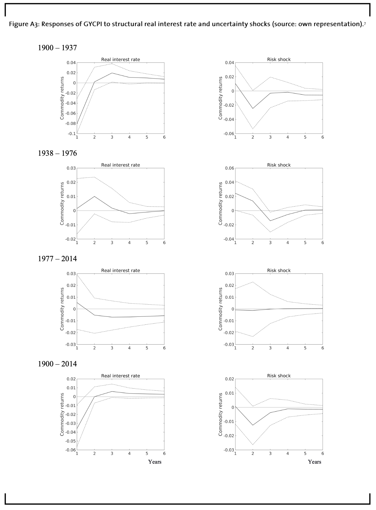
7The graphs show the response of the GYCPI to a generalized one standard deviation innovation in real interest rates and risk for different periods of time. Also shown are the 95% confidence bands based on 1000 Monte Carlo simulations.