Chemical industry activity as a leading indicator of the business cycle
Activity in the chemical industry has been found to lead that in the overall economy. The author constructs a Chemical Activity Barometer (CAB) that is a leading indicator which can be used to anticipate the peaks and troughs in the US economy’s business cycle. This article discusses the construction of the CAB and its performance. The results were robust and since 1919, the CAB was found to lead National Bureau of Economic Research (NBER) business cycle peaks by an average of eight months and troughs by an average of four months. In this time of such uncertainty, the CAB could be an important tool for economists, business analysts and anyone else trying to follow the US economy.
1 Introduction
In the study of economic fluctuations, many industries have been found to lead or lag the overall business cycle. When an industry (or some of its products) consistently leads the economy’s business cycle, a leading indicator or barometer can be developed from measures of that industry’s activity. The indicator can be used to assess turning points in the economy’s business cycle. These turning points are the business cycle peaks and troughs that the National Bureau of Economic Research (NBER) uses to identify the economy’s recessions and expansions or downturns and upturns. Activity in the chemical industry has been found to lead that in the overall economy. This paper provides an overview of a Chemical Activity Barometer (CAB) that is a leading indicator which can be used to anticipate the peaks and troughs in the US economy’s business cycle.
2 Business Cycle Indicators
The development of leading economic indicators of the business cycles has a long and interesting history. Business cycle indicators have proven to be useful tools for analyzing alternating sequences of economic expansions and contractions known as the business cycle (Persons, 1922; Wallace, 1927; Moore, 1980; and Moore 1990).
Business cycle indicators are based on business cycle theory that focuses on generally uniform sequences in economic activity noted by Wesley C. Mitchell (Mitchell, 1927). These sequences are revealed in statistical time series indicators that typically lead, coincide, or lag the business cycle. In its modern form, the approach can be traced to a list of business cycle indicators compiled by Wesley C. Mitchell (Mitchell, 1927) and then Wesley C. Mitchell and Arthur F. Burns for the NBER in the 1930s (Mitchell and Burns, 1938) and later refined in the 1940s (Burns and Mitchell, 1946). Indeed, much of the early research of the NBER focuses on developing a system of indicators to anticipate cyclical change in the economy as well as development of national income concepts and measurements. Geoffrey H. Moore built upon the research of Burns and Mitchell to develop the original index of leading economic indicators (LEI) for the United States (Moore, 1980). Thereafter, the business cycle indicator approach was further developed and refined. In 1961, the US Department of Commerce began publishing Business Cycle Developments, a monthly review of cyclical indicators identified by the NBER. The publication was renamed the Business Conditions Digest in 1968 and subsequently rolled into the Survey of Current Business (Niemira and Klein, 1994) that is still published by the Bureau of Economic Analysis (BEA). In 1995, this BEA cyclical indicators program was transferred to the Conference Board, a business membership and research association.
In order to emphasize the cyclical patterns inherent in the various individual cyclical indicators and de-emphasize the volatility of the individual indicators, the best of them are combined into composite indexes. Composite economic indexes can be leading, coincident, and lagging. They are essentially composite averages of several individual leading, coincident, or lagging indicators. They are constructed to summarize and reveal turning point patterns in economic data in a clear and convincing manner than any individual components as they smooth out some of the volatility of individual components (Burns, 1950; Zarnowitz, 1992). Use of these composite indexes is consistent with the historical view of the business cycle developed by Burns and Mitchell (1946). In particular, composite indexes can reveal common turning point patterns common to a number of cyclical indicators in a clearer and more convincing manner than the behavior of any individual indicators. Essential to understanding the business cycle is the ability to distinguish between leading, coincident and lagging indicators of the cycle, which essentially reflects the timing of their movements:
- Leading indicators (average weekly hours, new orders, consumer expectations, building permits, stock prices, etc.) are those that consistently turn before the economy does.
- Coincident indicators (employment, industrial production, personal income, business sales, etc.) turn in step with the economy and track the progress of the business cycle.
- Lagging indicators (inventory-to-sales ratios, change in unit labor costs, C&I loans outstanding, etc.) turn after the economy turns, thus playing a confirming role.
These three types of indicators are important in their own right although most attention is focused on the leading indicators because they tend to shift direction in advance of the business cycle. Leading indicators are better at calling the direction of the economy (contraction or expansion) than in predicting the pace of growth. This is based on economic theory first explained six decades ago at the NBER by Ruth Mack in her landmark study of the shoe, leather and hide industries (Mack, 1956). Although the use of composite economic indexes has existed for nearly three-quarters of a century, their use has been eclipsed by the more widespread use of structural econometric and times series analysis techniques. Nonetheless, composite economic indexes are still used by business economists and other analysts. Currently, the most prominent US composite economic indicators are those reported by the Conference Board, the Economic Cycle Research Institute (ECRI), and the Organization for Economic Co-operation and Development (OECD).
3 Constructing a Chemical Activity Barometer (CAB)
It makes sense that a composite index of chemical industry activity leads activity in the overall economy because the sector is affected first by underlying changes in the economic environment and its dynamics are determined partly by their position in the value chain. Since the chemical industry is a supplier to many other industries in the economy, it is highly vulnerable to inventory effects. These effects can occur if customers of chemicals place fewer orders in order to run down their own inventories. As a result, chemicals production tends to reveal cyclical developments at an earlier stage than other industries.
3.1 Various chemicals and plastic resins lead the cycle
The CAB is a composite economic index designed to be a leading indicator of broader economy-wide activity. Each component has a lead time that helps determine the direction in which the economy is heading.
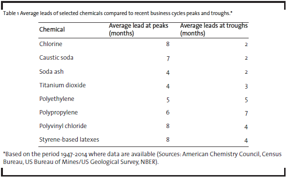
To analyze these leading properties of chemical production, the author examines the relationship between the cycles in the production of the selected chemicals in Table 1 (and other chemicals) and business cycles in the larger economy. The focus is set on the period from 1947 to 2012. As discussed above, many chemicals (and chemicals-related indicators) have features (or properties) that by their position in the supply chain lead the overall business cycle. For example, chlorine is an inorganic chemical product used as raw material starting block for polyvinyl chloride (PVC) resins. These PVC resins are used to manufacture a wide variety of plastic products for building and construction (siding, pipe, windows and doors, etc.), consumer and institutional, packaging, electrical/electronic OEM equipment (i.e., wire and cable) and other applications. Thus, production of PVC resins (and chlorine) could normally lead plastic products production, which in turn should lead home construction and production of a broad class of goods manufacturing. Activity in the chemical industry, which mainly produces intermediate goods sold to other manufacturing industries, correlates most closely with activity in the manufacturing cycle. The chemical industry is an early-cycle industry as it exhibits its turning points in the business cycle earlier than the overall manufacturing industry and the overall economy. This also holds true for plastic and rubber products, the chemical industry’s prime enduse customer industry. For recent business cycles, Table 1 presents the average lead (in months) in the production of a number of chemicals compared to NBER business cycle peaks and troughs. The data represent averages as the variance of leads for any one chemical individually can be large. In PVC resins, for example, leads at peaks were as short as two months or as long as 17 months. In some cases, no lead was provided (PVC in the 1991 trough) or even lagged the overall business cycle (by one month at the 1991 trough for chlorine). Despite just-in-time inventory management, the average leads did not appreciably change during this six decade period.
3.2 Theory behind developing a composite index
The results of this investigation of data (and leads and lags) were eventually used to develop a leading economic index (or barometer), the CAB. The performance of single indicators in any given period is likely to vary due to which causal forces are dominant. Some leading indicators may perform better in some conditions and other indicators in differing conditions. Individual times series, for example vary in timing and smoothness. No single leading indicator of an economic process or leading indicator system based on a product is perfect and some measure of protection against changes in leads and lags, and surprises of individual cases is needed. This can be accomplished by combining several leading indicators into one leading composite series (Burns, 1961). To improve the chances of getting true signals and reduce those of getting false signals, economists rely on a broad group of leading indicators and combine these into an appropriately constructed composite index (Zarnowitz, 1992). Due to diversification of many indicators, a composite index of leading indicators should work better over time than single indicators. Even with this methodology, a composite indicator can still engender false signals. Decision rules need to be developed in order to screen the information and determine cycle turning points signaled by a composite leading index. In addition, there need to be periodic reviews of the cyclical indicators used to construct the composite leading index to ensure the indicators still lead and are representative of the economic process and its place in the supply chains as well as add or substitute new indicators to the composite (Niemira and Klein, 1994).
Understanding the role of the chemical industry in the manufacturing industry and in the overall economy provides the foundation for developing a leading barometer of the business cycle using data on chemical production and other chemicalsrelated indicators. Useful leading economic indicators (or barometers) reflect economic relevance, they can be collected and processed in a statistically acceptable manner, they are fresh and not subject to frequent revision, they do not fluctuate erratically from month to month, they move reliably with general business activity, and they exhibit a consistent pattern over time as a leading indicator. By combining a number of indicators to create one composite barometer, the Chemicals Activity Barometer (CAB), addresses these criterion.
3.3 Constructing the CAB
To construct the CAB, a number of chemicals (and chemicals-related indicators) are evaluated. The indicators finally included in the composite encompass a weighted average of the production of chlorine and other alkalis, titanium dioxide and other pigments, PVC and other plastic resins (i.e., a mix of chemical products production); chemical prices; hours worked in chemicals; chemical company stock prices; end-use (or customer) industry sales-to-inventories; and several broader economic leading economic measures (building permits and Purchasing Managers’ Index of the Institut for Supply Management (ISM PMI)). High frequency data such as chemical railcar loadings, prices, and equity prices are used to extend the CAB for the current month.
Some challenges posed in developing the CAB include issues with consistency in the underlying time series over the time period. For example, the transition from the SIC to the NAICS nomenclature presents consistency challenges. In some cases, monthly production data are not available for the entire period and an industrial production (IP) index that measured the approximate activity is chainindexed and employed to extend the data. In other cases, alternative measures are employed such as chain-indexing to expand a time series. For example, the S&P index for chemicals only goes back to January 1990. Its composition differs from that of another index used from January 1946 through December 2001. The latter, for example, is chained with the newer index to create one continuous index (or times series). Similar procedures are employed in dealing with production data.
There is a distinct break in the data used in constructing the CAB in the period prior to 1946. The production-oriented data simply changed through time due to reporting changes in government and trade association statistical programs. Some of the physical production data (e.g., chlorine) are available back to the opening months of World War II but there was generally a paucity of data. In addition, many of these products went through different stages of the product life cycle. A plastic resin such as low density polyethylene, for example, would have been considered a specialty, high-performance product in the 1940s but by the 1960s would have been considered a commodity.
An older monthly Federal Reserve Board chemicals production index (with a base year of 1935-39 average = 100) is available back to 1923 and monthly data are available for other products (e.g., wood alcohol or methanol) and used to create production indexes to represent chemical industry output back to 1918. Along with consistent price and other data this is used to extend (via chain-indexing) the CAB back to 1918. The collecting of data provides unique insight into the changing structure and composition of industry.
Using the times series data discussed above, the CAB is constructed using a five-step procedure similar to that used by the Conference Board’s to calculate composite indexes. This is a non-model approach and the steps are:
- Calculate month-to-month changes in the component indices;
- Adjust month-to-month changes by multiplying them by the component’s weighting;
- Sum the adjusted month-to-month changes (across the components for each month);
- Compute preliminary levels of the composite index; and
- Rebase the composite index to reflect the average lead (in months) of an average 100 in the base year (the year 2007 was used) of a reference time series (the Federal Reserve’s Industrial Production index was used1).
1The Federal Reserve Board’s headline industrial production index was used as a reference time series due to its consistent coverage back to 1919.
To update the CAB from month to month, steps 1 through 4 are followed to incorporate the most recent six months of data. The revisions to the base year (step 5) are made when the Federal Reserve changes its base year for the industrial production (IP) index.
To determine business cycle peaks and troughs, the NBER examines and compares the behavior of various measures of broad activity: real GDP measured on the product and income sides, economywide employment, and real personal income. The NBER also may consider indicators that do not cover the entire economy, such as real business sales and the Federal Reserve’s index of industrial production (IP). For the purposes of this analysis, the industrial production index was used as a reference time series due to its long history and consistency.
Analysis of the data indicates a positive correlation of over 0.90 between the industrial production index and the CAB eight months prior. There is also a high correlation between real business sales and the CAB. More interesting is how the average leads have changed through time.
Table 2 presents the timing relationship (in terms of months of lead) between the CAB and the overall business cycles since 1919. The findings should be viewed in perspective, insofar as not every cycle in industry proceeds uniformly. When comparing the chemical industry and overall business cycles, the respective intervals of the turning points can vary substantially. The data presented in Table 2 indicate that the chemical industry’s lead time can vary. The CAB provides a longer lead (or performs better) at business cycle peaks, leading by two to 14 months, with an average lead of eight months. The median lead was also eight months. At business cycle troughs, the CAB leads by one to seven months, with an average lead of four months. The median lead was also four months. In the most recent business cycle, the CAB led the peak by five months and led the trough by three months.
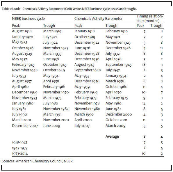
Examining the data in Table 2, the author divided the 1918-2014 period into 3 roughly three-decade periods to examine how the average leads changed. The first period represents a period that was characterized by two world wars and the Great Depression and one in which data availability was scarce. The second period from 1947-1973 reflected a period in which US data quality improved and was broadened and one in which was characterized by the Post World War II boom. The years 1973 was chosen as it represented the first oil price shock and the end to the boom. The period from 1973 represented a period characterized by several oil price shocks, the Great Moderation, and lastly the financial crisis and the Great Recession. The data indicate that there was little difference between the first and second periods in terms of average leads at peaks and troughs. There was, however, a distinct change with the third period. In the third period, the average lead at peaks improved, from seven months to 10 months. At the same time, the average lead at troughs deteriorated, from five months to two months.
The CAB is not a leading index of chemical industry activity. Rather, it is a leading index (barometer) based on chemical industry data that leads overall industrial production and the overall business cycle. The relationship between the CAB and IP index are presented in Figures 1 and 2. Figure 1 presents the CAB versus the IP index and Figure 2 presents the year-over-year growth rate of the CAB and the IP index for the 1948 through 2014 period.
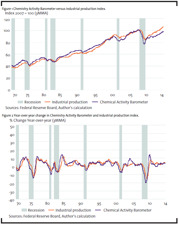
The data for both are available back to 1919. The shaded columns in both charts represent periods of recessions. The data presented in both figures are based on three-month-moving averages to smooth volatility and thus ease comparisons.
The predictive value of the CAB or other leading indicators is limited by the weight assigned to its component indicators to distill information in each into a single variable, and the varying degree of efficacy of those indicators over differing time horizons. As a result, leading indicators can sometimes provide false signals indicating early peaks (or early troughs). This is especially the case with a composite indexes based on a limited number of underlying indicators, some of which are correlated. A decision rule is needed. For purposes of this analysis, a false signal is defined as periods where the indicator declines for three or more consecutive months and that the decline in the leading indicator (in this case the CAB) exceeds 3% from peak to trough but that an official recession (as per NBER) does not occur. As Figure 2 illustrates, the early supply chain position of the chemical industry makes it vulnerable to wide swings of production activity. This is especially the case with individual products; a main reason why a composite index of activity is used. Swings of ±10% are not unusual and the criteria suggested above represent a low bar. Using this decision rule and examining the CAB performance, however, a false peak has only occurred once (in March 1966 when a false peak occurred in connection with a “growth recession” at that time). At other times (March 1984, June 2002, April 2006, April 2010, and March 2011) slowing activity was signaled with three or more consecutive months of slight to modest decline. Even less pronounced were several two-month slowdowns flagged in July 1951, December 1955, and January 1995. When taking a higher percentage limit for decline, no false signals emerge.
The CAB estimate for any given month can be released by the fourth week of that month as sufficient high-frequency data are available for that month. The monthly CAB estimate is subject to revision (reflecting revisions in the underlying data). This is particularly the case of the CAB released during the current month using high-frequency data. But because of the nature of the underlying price, equity and production data, non-benchmark monthly revisions are generally minor once the current month CAB reading is revised during the subsequent month.
4 Summary
Due to the chemical industry’s early position in the supply chain, the CAB is useful in determining future trends in the overall business cycle and the overall US economy. The CAB is particularly useful in indicating business cycle peaks and in signaling the phase of the business cycle in which the economy is heading. The CAB is a valuable tool that can be used by business journalists, business economists, policy advisors, security analysts, and others interested in assessing the future direction of the US economy.
This approach could be extended to the EU and other nations and regions but due to the paucity of data, the time period would be shorter. For the EU28, for example, quality consistent data may only be available back to 1990. That said, the approach could be applied to nations such as Canada and the United Kingdom that do have extensive indicator data for a long time period.
References
Burns, A. (1961): “New Facts on Business Cycles”, in: Moore, G. (ed.) Business Cycle Indicators, Vol. 1. Princeton University Press: Princeton, NJ.
Burns, A., Mitchell, W. (1946): Measuring Business Cycles, National Bureau of Economic Research: New York, NY.
Mack, R. (1956): Consumption and Business Fluctuations: A Case Study of the Shoe, Leather, Hide Sequence, National Bureau of Economic Research, New York, NY.
Mitchell, W. (1927): Business Cycles – The Problem and Its Setting, National Bureau of Economic Research, New York, NY.
Mitchell, W.,Burns, A. (1938): Statistical Indicators of Cyclical Revivals, Bulletin 69, National Bureau of Economic Research, New York, NY.
Moore, G. (1980): Business Cycles, Inflation, and Forecasting, Ballinger Publishing, Cambridge, MA.
Moore, G. (1990): Leading Indicators for the 1990s, Dow Jones-Irwin, Homewood, IL.
Niemira, M., Klein, P. (1994): Forecasting Financial and Economic Cycles, John Wiley & Sons, New York, NY.
Persons, W. (1922): Measuring and Forecasting General Business Conditions, American Institute of Finance, Boston, MA.
Wallace, W. (1927): Business Forecasting and its Practical Solution, Pitman & Sons, Ltd., London, England.
Zarnowitz, V. (1992): Business Cycles – Theory, History, Indicators and Forecasts, University of Chicago Press, Chicago, IL.