Standardized cost estimation for new technologies (SCENT) – methodology and tool
Abstract
This paper presents the development of a methodology and tool (called SCENT) to prepare preliminary economic estimates of the total production costs related to manufacturing in the process industries.
The methodology uses the factorial approach – cost objects are estimated using factors and percentages on the basis of the purchased equipment cost. The chosen approach is based on an extensive literature survey on methodologies and suitable data. The approach has the advantage that it can be based on a limited amount of data (list of equipment required for the technology). Therefore it is especially suitable for new or emerging technologies. The theoretical accuracy of the prepared estimates is within ±30%.
1 Introduction
Ever since the industrial revolution the process industries have played an important role in improving the quality of human life. Over the last 200 years, the process industries have gained significant importance in society by introducing products that dramatically changed the world. Key examples are pharmaceuticals, food products, and food additives, fuels, and polymers. At the same time, many technologies have led to controversial societal discussions, leading to the quest for a holistic technology assessment. There is a wide consensus that the three sustainability dimensions–economy, environment, and society – need to be taken into consideration when assessing a technology.1 This paper deals with the (micro-)economic assessment, with the goal of preparing a readily applicable tool-set for the economic evaluation of new and emerging technologies.
In today’s world, the economic performance is a conditio sine qua non for the existence and the future application of technology. New technologies resulting in better, more environmentally friendly products are often more costly. The additional costs might be caused by higher capital investment (e.g. due to improved heat integration or measures for environmental or health protection) and/or higher operational costs. Decisionmaking sometimes implies a trade-off between environmental or social benefits and economic costs. Therefore, careful and precise assessment of all costs related to technology is of great importance to determine the prospects of technology.
It is evident that there is a strong need for a reliable estimation of the full costs of a product on the micro level (“small” in Greek; refers here to the costs of a single manufacturing plant). These costs include many components, most of them not easy to forecast and calculate – capital investment in equipment and buildings, expenses for maintenance and repairs, materials and energy costs, salaries for employees.
Different approaches exist to obtain these data. For currently existing technologies, a relatively easy and trustworthy method is the comparison of historic real plant data. Many manufacturing processes have existed for more than 50 or 100 years and tens and hundreds of similar plants have been built on the planet. Such data are, however, not easily available due to their confidential and proprietary nature(e.g. Dysert, 2003). Moreover, when assessing new technologies, it is a further challenge, that historic data is typically of no or only very limited use.
Very often, estimates are made using complex commercial software tools.2 These tools may require a large amount of input data which are not always available for new technologies. Extensive previous knowledge and training on the software is also necessary. The commercial nature of the tools makes it difficult to compare estimates made by application of different tools. The need to rely on the outcome of one single tool is therefore quite common.
When preparing an economic analysis for new technologies, up-to-date data on prices are needed for many items, such as equipment, instrumentation and controls, chemicals, utilities (electricity, water, and natural gas), salaries for operating and skilled labour. One can obtain this information from vendors, suppliers, manufacturers, government statistics offices and others. All this requires significant effort. Unfortunately, there is no unified database which contains all necessary information for preparing basic cost estimates. Such a database was published in the open literature for the last time in 1990 (Couper, 2003).
There is hence an urgent need for a publicly available estimation method, which could provide sufficiently accurate results. It is apparent that in early stages of the development of new technologies, only study or preliminary estimates can be made. Despite the great deal of uncertainty existing for new technologies, the basic information required for conducting a cost analysis is often rather well known: this includes material balances (raw materials, solvents, catalysts), major pieces of equipment, important service facilities (e.g. steam generation) and energy balances (use of
Consequently, the question addressed by this study is how to use this information to arrive at reliable cost estimates for (new and emerging) technologies, thereby making use of existing cost estimation techniques. By conducting a literary survey covering different types of process cost analyses this paper pursues the following goals:
- To develop a cost estimation methodology to be used as standardized, default approach when making economic analysis for new or emerging technologies.
- To compile a database of all relevant costs and expenses necessary to prepare a study or preliminary estimate for a new technology; these include, for example, prices of major types of equipment, utilities, chemicals, environmental protection expenses and labour costs.
- To combine the methodology and the database into a simple cost assessment tool which would allow a quick and handy estimation and which can also be performed without previous specific expertise in cost estimation.
Many publications (mostly handbooks) deal with economic aspects of plant and process design, but most of them refer to just a handful of authors. From the literature review we performed we concluded that the most authoritative authors dealing with capital investment and production costs estimates are Peter, Timmerhaus and West (2004) as well as Couper (2003 and 2008). This paper is based mostly on their work but we have also accounted for the work of a few other authors (see section 3 “Essence of the factorial methodology”).
2 Classification of the production costs
The classification in this study is mainly based on the work of Peters, Timmerhaus and West (2004). Their classification is the most comprehensive, includes most examples and was updated very recently. They are considered authorities in this area and many other publications refer to them. One important point made by them is that the main source of inaccuracy in economic estimates is actually not under-estimating or over-estimating individual data inputs rather than missing a cost object. Therefore the classification is of lower importance than the diligent application of the tool, thereby avoiding omissions.
The classification presented in this paper (see below) exhibits an intermediate level of detail. In contrast, more elaborate classifications are applied when preparing detailed estimates. Examples of elaborate classifications are given by Couper (2003 and 2008) and by Holland and Wilkinson (1997).
Production costs are the costs required for the plant to manufacture a product and they are expressed either per unit(s) produced (e.g. per tonne of product) or on basis of time: hourly, daily, monthly or annually. In effort of standardization, we recommend to express the production costs on an annual basis because it covers for seasonal variations in expenses, sales and process conditions as well as planned maintenance and shut-down periods.
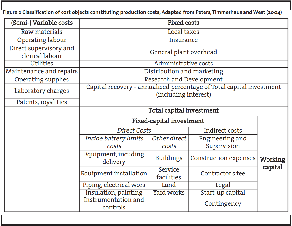
The production costs are generally classified as (semi-) variable and fixed costs. The variable costs are proportional to the load factor of the manufacturing, while fixed costs are independent of the plant capacity. Some of the variable costs are referred to as “semi-variable” because they have a minimum fixed component in them. The full list of production costs is given in Figure 2.
One of the most important fixed cost objects is the capital cost which includes all the buildings, machinery and equipment necessary for every-day operations of the plant. The initial capital investment (which may easily exceed $US 50 million for a large-scale manufacturing process; Peters, Timmerhaus and West, 2004) is recovered on annual basis through depreciation, with the depreciation regime being determined by tax laws. The annual cost is referred to as capital recovery cost, which is a fixed cost. The capital investment is generally classified in two main parts: the fixed-capital investment and the working capital.
The fixed-capital investment is all capital “fixed” to the ground, essentially tangible properties: e.g. equipment, machinery, buildings, and land. Since it may be as high as 80% of the whole capital investment (Peters, Timmerhaus and West, 2004) this cost might pre-determine the profitability of a technology and is a key factor in the decision making for a prospective investment.
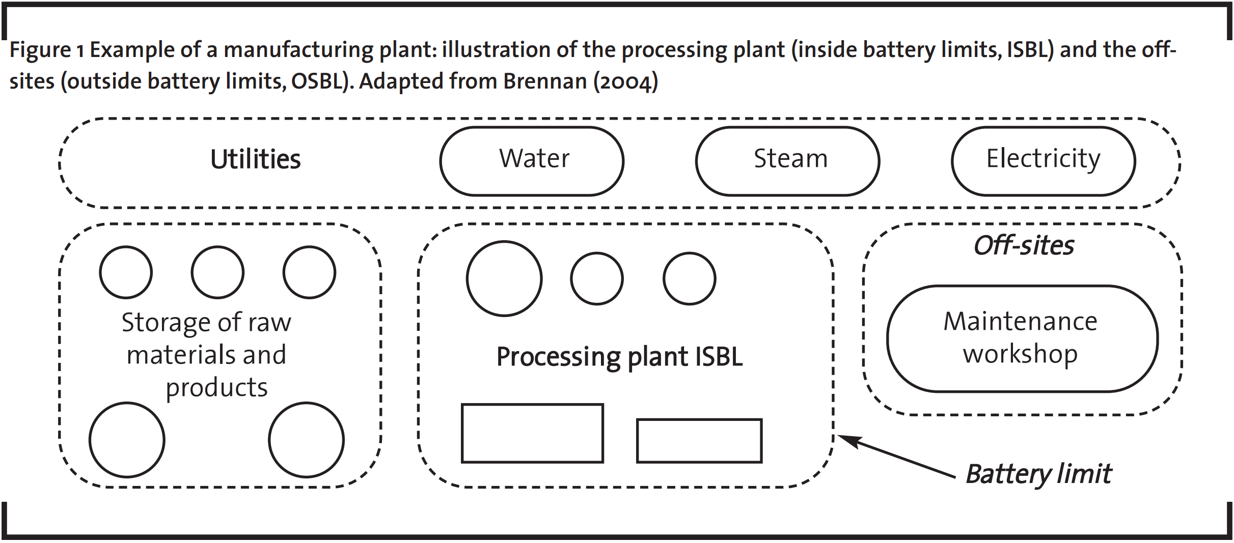
For process industry plants, the fixed-capital investment can be divided in two parts: inside battery limits (ISBL or IBL) and outside battery limits or off-sites (OSBL or OBL). Battery limit is a real or imaginary geographical boundary around an area in the processing plant where the actual manufacturing takes place (the conversion of the raw materials or intermediates into the product). Thus the inside-battery limits costs may be defined as all expenses for equipment, including delivery, installation, foundations, structures, piping, electrical works, painting, insulation as well as the cost incurred for instrumentation, control equipment and operation. All these are direct costs. One could say that the battery-limits is a subsystem of the plant, with the raw materials (or intermediates) and the utilities flowing in and the products flowing out (Figure 1).
Next to direct costs also indirect costs are applicable to the battery-limits, such as engineering and design expenses, construction costs, etc. These costs are typically charged to the project as a whole and cannot be assigned to specific cost objects. A list of the indirect costs is given in Figure 2. They normally include engineering and supervision expenses, construction costs for the project including the contractor’s fee and all costs required to meet the legal requirements for building the plant. There is an additional “allowance” called contingency capital which is usually a percentage of the value of the whole project. This capital is meant to cover any unforeseen events, such as unpredicted delays due to weather conditions, strikes, transportation issues, etc.
The other direct costs (or the outside-battery limits costs) are expenses for land, yard improvements such as fences or roads, various buildings and service facilities (e.g. boilers, cooling towers, facilities for compressed air or steam generation). The latter are commonly referred to as “off-sites”.
For every enterprise, there is also a sum of money required to conduct everyday operations. It is necessary to cover expenses such as salaries, utility bills (electricity or natural gas), to regularly purchase raw materials and other supplies. This sum of money is called the working capital and it is not available for another purpose; therefore it is regarded as an investment item and is part of the capital investment.
Working capital is defined as the total amount of money invested in: raw materials and supplies in stock; finished products in stock and semi-finished products still in process of manufacturing; cash required for regular payments of operating expenses (salaries and other bills for a limited period); accounts receivable; accounts and taxes payable (Peters, Timmerhaus and West, 2004).
It is important to realize that even though operating expenses such as salaries, raw materials supply and others are taken into consideration in the working capital, the working capital is not an operating expense but that it is instead part of the capital investment. It is used to ensure liquidity of the firm. The reason behind this is that a company will have to constantly maintain cash to cover its everyday expenses.
The working capital is constantly regenerated with income from sales and stays at roughly the same level throughout the plant’s lifetime. The working capital is by far smaller than the sum of all operating expenses for the whole year. It typically allows covering for one or two months of salaries, few months of raw materials supplies and other operating supplies. All this depends on the specifics of the business and the regularity of payments. It is also largely dependent on sales: seasonal sales will lead to less regular re-liquidation of the working capital and therefore, higher working capital will be required.
To facilitate the estimation of production costs, the SCENT tool (Standardized Cost Estimation for New Technologies) was developed. It has been prepared in the form of MS Excel file and is organized according to the classification presented above. It incorporates all equations and correlations between the cost objects which will be discussed in the further course of the paper. It follows a simple approach using drop-down menus and pre-defined values which allow usage without previous economic training.
3 Essence of the factorial methodology
Based on a literature review it can be concluded that preliminary cost estimates are usually based on the cost of the purchased equipment, with all additional cost objects being estimated by means of specific default “factors”, i.e. certain percentages of the purchased equipment cost. The accuracy of the estimate will vary depending on the level of detail known about the design of the plant. In early stages of the projects only preliminary estimates can be made. In later stages when there is more information about equipment requirements and the design specifications, more accurate estimates are possible (Towler and Sinnott, 2008). Important consideration is also the qualityof the cost data (especially prices and scaling up or down for the specific technology). From the preliminary flowsheets the pieces of equipment are selected and the purchased equipment cost is estimated. Usually prices of equipment are given by manufacturers and vendors as f.o.b..3 Delivery charges and installation expenses should then be added. The best source for this information are the manufacturers and sellers of the equipment, however, for preliminary estimates, such quotations might be too difficult or time intensive to obtain (we have therefore compiled default data in the SCENT tool, see below).
From the cost of the delivered equipment the fixed-capital investment is determined. Once the fixed-capital investment has been estimated it is used as a base for estimating other costs: by multiplying the fixed-capital investment with different factors, one can obtain an estimate of the working capital and few major cost objects: e.g. maintenance, insurance, taxes and others (see below).
There are some costs which cannot be estimated on the basis of the purchased equipment cost or the fixed-capital investment since there is no correlation between them. Examples are the costs for raw materials and utilities. Those expenses are estimated from the material and energy balances (raw materials demand, utilities) and the respective prices or directly from the specifics of the technology (e.g. environmental expenses).
Towler and Sinnott (2008) give a short summary of the steps that need to be taken to make an estimate using the factorial methodology. The steps used in the SCENT tool follow a similar pattern (as mentioned above SCENT also contains databases on prices and estimation factors):
- From the preliminary flowsheets the estimator should identify the pieces of equipment required, together with specifics such as their capacity, material of construction (e.g. stainless steel versus regular steel), additional concerns such as extreme pressures or temperatures, etc.
- Determine the purchased costs and – by multiplication with equipment installation factors – estimate the installed cost for each piece of equipment (see below for further explanation)
- Estimate the fixed-capital investment including all direct and indirect costs
- Based on the fixed-capital investment estimate the working capital
The approach presented so far leads to the estimated total capital investment (see Figure 2). This cost occurs at the beginning of the project, depending on the time required for planning and construction. Afterwards, the actual manufacturing of the product starts and the total capital investment is gradually recovered. The capital recovery is included in the total production costs by application of the annuity method (see below). Production costs can be expressed as costs per year (or other time frame) or costs per unit of product (e.g. per tonne of product). For the reasons given above we determine in SCENT the costs per year.
- Based on the material and energy balances, estimate the raw materials (chemicals, solvents), utilities (water, electricity) and expenses for environmental measures
- Estimate the labour costs
- Estimate the total production costs including all (semi-) variable and fixed costs
The most significant and also most difficult part in this process is the estimation of the fixed capital investment. It relies mainly on the accuracy of: the input cost data of the purchased equipment, the installation factors used to account for the installation of the equipment (see below), and the correlation factors to account for all other direct and indirect costs (buildings, engineering, etc.). According to Peters, Timmerhaus and West (2004) the first two items may reach 80% of the fixed-capital investment. The equipment installation factors account for installation material and labour, foundations, structures, piping, fittings, electrical works, painting, insulation. Depending on the source of the factors, they might also include the required instrumentation and controls and might be based on the purchased equipment cost (f.o.b.) or on the delivered equipment cost (including freight charges). The value of the installation factor is always > 1, resulting in theinstalled equipment cost when multiplied with the purchased equipment costs. The accuracy of the input data can be increased by acquiring more recent, up to date information on the purchased cost of the equipment used. Many of the other cost objects are based on these cost data. Therefore increasing its accuracy will ultimately increase the quality of the final estimated cost. The best quality can be achieved by getting exact quotes from equipment manufacturers or suppliers – these are always recent, and will be chosen in accordance with the technical requirements of the process.
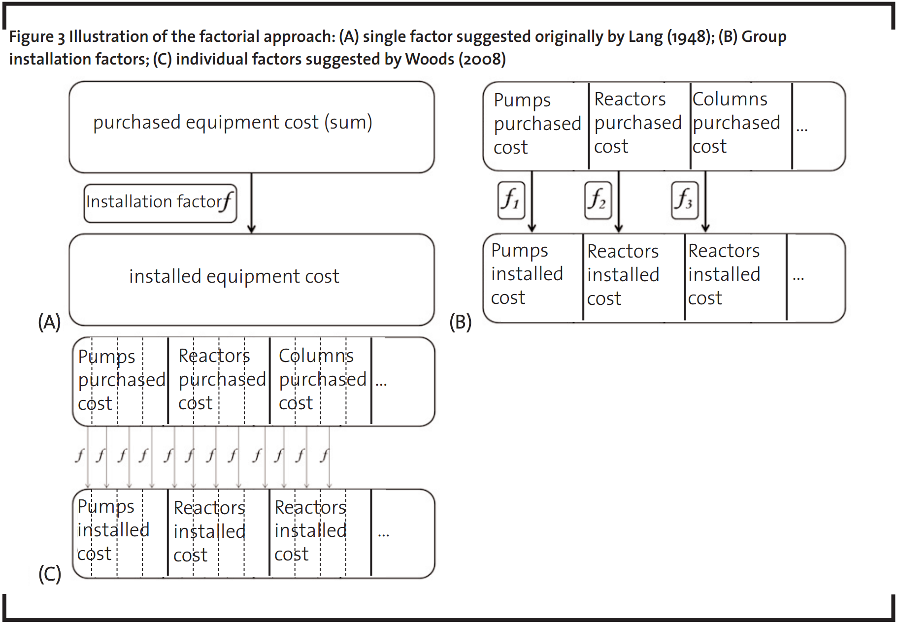
This factorial approach was first suggested by Lang in 1948. He differentiated between three types of processing plants: solid (e.g. a coal briquetting plant), solid-fluid (e.g. a shale oil plant with crushing, grinding, retorting and extraction) and fluid processing (e.g. a distillation separation system)4 and accordingly suggested three types of installation factors. He proposed the sum of all purchased equipment cost to be multiplied with the corresponding installation factor to yield as a result the sum of the installed equipment cost. This approach is illustrated in Figure 3(A).
Later on, these factors were refined by several authors (e.g. Hand, Wroth, and Guthrie (as quoted by Couper (2008)) and more specific “group installation factors” 5were developed as illustrated in Figure 3(B). More recently, individual factors have been developed. These installation factors are strictly specific for each individual type of equipment: i.e. two different types of pumps have different installation factors in contrary to the group factors where all types of pumps have the same installation factor. These factors are typically much more accurate than the previously presented methods. Woods (2008) gives a detailed list of about 500 different pieces of equipment, each along with individual installation factor. The individual factor approach is illustrated in Figure 3(C).
In the SCENT tool it was decided to use the individual equipment installation factors by Woods (2008) for the following reasons:
- Higher accuracy – the individual factors are more specific
- Most recent – they were first published in 2007 and re-printed in 2008
- Woods’ approach deliberately excludes instrumentation and controls from its factors while earlier factors include it. The reason behind the exclusion is that instrumentation and controls has undergone major development and accounting for them in a simplistic way by means of a default factor could therefore cause inaccuracies.
- Detailed – Woods also gives capacity exponents, alloy correction factors and additional correction factors for the temperature and pressure level and other process conditions which are all specific for each individual piece of equipment. This gives the estimator the opportunity for higher level of customization, and better accuracy of the estimate
- Labour / material ratio – Woods gives the ratio between the costs for labour and material which are incorporated in each installation factor. This makes it possible to correct in SCENT for the location by country, as will be described in detail in the next section
For all other cost objects in the capital investment and the production costs (e.g. offsites and maintenance) mainly Peters, Timmerhaus and West (2004) are used as a source for few major reasons:
- Authoritative – the publication by this group of authors has been updated regularly and recently (2004). It has been referenced by many other authors working on the topic of cost estimation.
- Most consistent – many authors present factors to estimate certain cost objects, but the most comprehensive approach proved to be the one by Peters, Timmerhaus and West.
- Additional considerations – this group of authors presents additional considerations and different values for some of the cost objects (for example, they suggest three different values for buildings depending on whether a new plant is built on an undeveloped site or on an existing site or whether it is simply a small expansion on an existing site). These considerations allow for higher accuracy of the estimate. They will be presented in greater detail in the next section.
4 Cost estimation
The process industries represent capital intensive sectors (Economy Watch, 2010). Therefore, the accurate estimation of the capital investment is of crucial importance. When presenting the methodology the capital investment estimate will be discussed first, partially because it is the first step in project development but more importantly because the value of the capital investment is necessary to estimate other cost objects (e.g. the maintenance and repairs expenses).
4.1 Capital investment estimate
4.1.1 Purchased Equipment
In the SCENT tool the cost data by Woods (2008) have been implemented with all prices given f.o.b. in US $. The purchased equipment cost calculated by the tool includes in total all pieces of equipment from the process flow sheet, spare parts, surplus equipment, supplies and equipment allowance.
All prices in this database refer to a value of the Chemical Engineering Plant Cost Index (in short: CEPCI) of 1000. The CEPCI value for the years 1957–1959 was 100 while the value for 2010 was 585.9. By choosing today’s (or an expected future) CEPCI value in SCENT, the results are adapted to the respective price levels. The CEPCI index is published at the end of each month in the Chemical Engineering magazine (Dysert, 2003).
The prices taken from Woods (2008) were published in the year 2007. In combination with the newest CEPCI values they allow to generate estimates with good accuracy also for a limited period in the future by using these historic cost data. Couper (2003) suggests that it is acceptable to use the same cost data with the correction of a cost index for no longer than 10 years.
All prices in this database are given as base cost with a base capacity. The database also contains equipment-specific scaling exponents which allow estimating the cost of a given piece of equipment with a different capacity:

In case the scaling exponent is unknown, a value of 0.6 or 0.7 can be used as default (also referred to as six-tenths or seven-tenths rule). Equation (1) represents the economies of scale because buying a piece of equipment with twice the capacity is less than twice as expensive (when the exponent is less than 1.0). If, for a specific piece of equipment, this exponent is larger than 1.0, the most cost-effective way of scaling up is to duplicate the equipment. In the SCENT tool, a valid equipment-specific capacity range is suggested to the estimator.
Most of the equipment is offered with standard material of construction, usually cast steel (c/s) or cast iron. If special construction is required (e.g. stainless steel (s/s), nickel or any type of alloy), an alloy factor is applied to estimate the cost of the equipment. The alloy factor is specific for each type of material and equipment. Multiplication of this alloy factor by the cost of the equipment made of the standard material yields the cost of the equipment made from the chosen material as shown in equation (2).
Additional factors are provided to estimate the cost of equipment working at different process conditions or with different specifications: e.g. factors for elevated temperature or pressure. The approach is the same as with the alloy factors: the base cost of the equipment is multiplied with the additional factor (equation (2)). These factors are individual for each type and subtype of equipment (e.g. individual factors for pumps depending on the working pressure).

Delivery charges for transportation, freight insurance, duties, and taxes are not accounted for by the installation factors. This cost may vary significantly depending on the plant’s location or government regulations. Such estimation is hard to make in a very early stage of the project because the manufacturer or the vendor of the equipment might be yet uncertain as well as the plant’s location might still be in question. Therefore, for preliminary estimates, 10% of the purchased equipment cost is proposed as an average, standardized value as delivery charge (Peters, Timmerhaus and West, 2004). The purchased equipment cost including charges for delivery will be referred to as “delivered equipment cost”.
4.1.2 Installed Equipment
The installation factors account for installation material and labour, foundations, structures, process piping, pipe fittings, valves, painting, insulation, electrical systems and equipment switches, motors, feeders, grounding, wiring, lighting, panels, etc. The installation costs are estimated using equation (3):
![]()
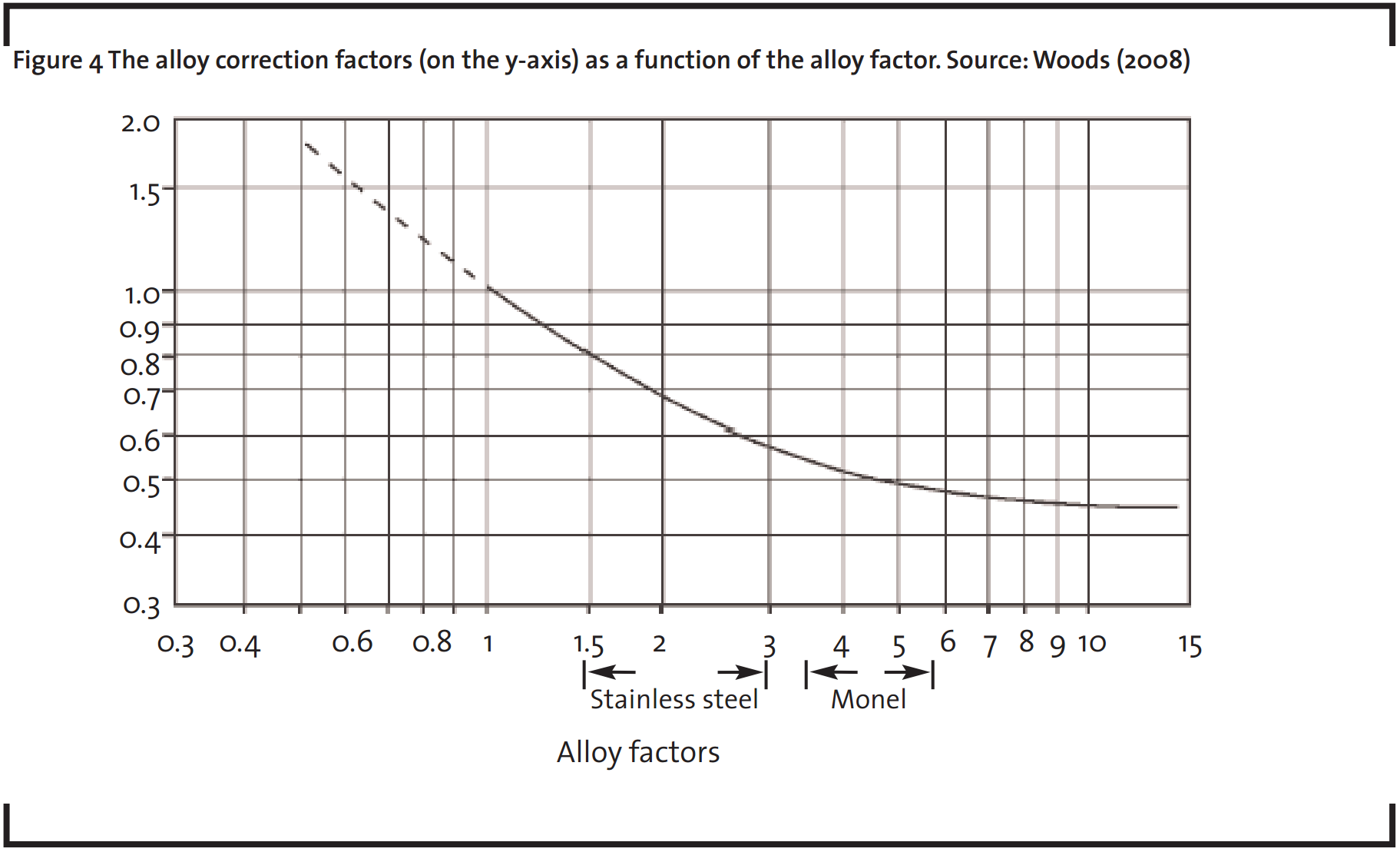
When the installed cost is estimated for equipment made of more expensive alloys, equation (3) needs additional correction because labour will generally be the same, structures and foundations will be mostly the same and also the expenses for electrical works might not be affected. When estimating equipment made of special materials, equation (3) therefore leads to overestimation. To correct for this, an alloy correction factor is applied according to equation (4):
![]()
The alloy correction factor is applied only when the installed cost is estimated and only when beforehand an alloy factor was used to estimate the purchased cost. The alloy correction factor is presented separately from the alloy factor, because it is only applied to the installed cost (this explains multiplication by the term (fINST-1) in equation 4), while the alloy factor is used to estimate the purchased cost of the equipment.
The alloy correction factor was introduced by Brown (2000) as modification to Hand’s factorial approach (1958). The relation between the alloy correction factor and the alloy factor is given in Figure 4.6 It is logical that the higher the alloy factor, the higher the necessary correction is. In the figure the typical ranges for stainless steel and Monel alloy factors are presented, the exact values, however, remain specific for each type of equipment.
As mentioned above the installation factors presented by Woods provide the ratio between the labour and the material for each individual installation factor. This ratio could not be found in earlier publications. Using this ratio it is possible to develop simple country-specific factor to account for differences in labour costs in the various countries. The installation factor is split into two sub-factors, one for materials and one for labour costs as shown in equation (5):

There are always differences between the installation and construction costs in different geographical locations (countries). Two important assumptions were made:
- Most of the large equipment, as used in the process industry, is globally traded. It is therefore justified to use uniform international prices for purchased equipment. In contrast, the labour costs related to installation and operation may differ significantly between countries and sometimes even within a country. To correct for this, SCENT assumes that the difference in costsbetween geographical locations (countries) is driven mainly by the difference in the labour rates (while the fluctuations in material prices were assumed to be negligible).
- The installation factors suggested by Woods are based mainly on US data; they take into consideration the US labour rates. When a piece of equipment is installed in the USA, the cost should be accurate; however, when the same piece of equipment is installed outside the USA, the estimation might differ; it is assumed that this difference is driven solely by the difference in labour costs and therefore, a correction for this labour cost difference is applied.
Differences in labour costs are taken into account by introducing a correction factor which is applied only to the labor part of the installation factor. Subsequently, equations (3) and (5) are expanded into equation (6) to include this correction:

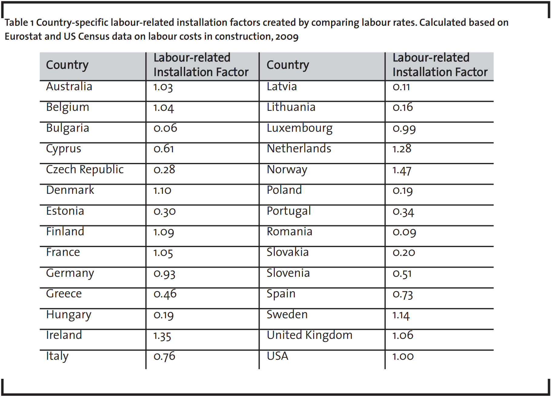
Country-specific labour-related installation factors were created by normalizing the values for all European Union countries (plus Norway) relative to the factor for the USA which is 1.00 (Table 1). The country-specific factor indicates whether the installation of a piece of equipment is cheaper or more expensive compared to the USA, only from labour point of view. When this factor is multiplied with the labour component of the installation factor, it will decrease or increase the total cost.
4.1.3 Fixed-capital investment
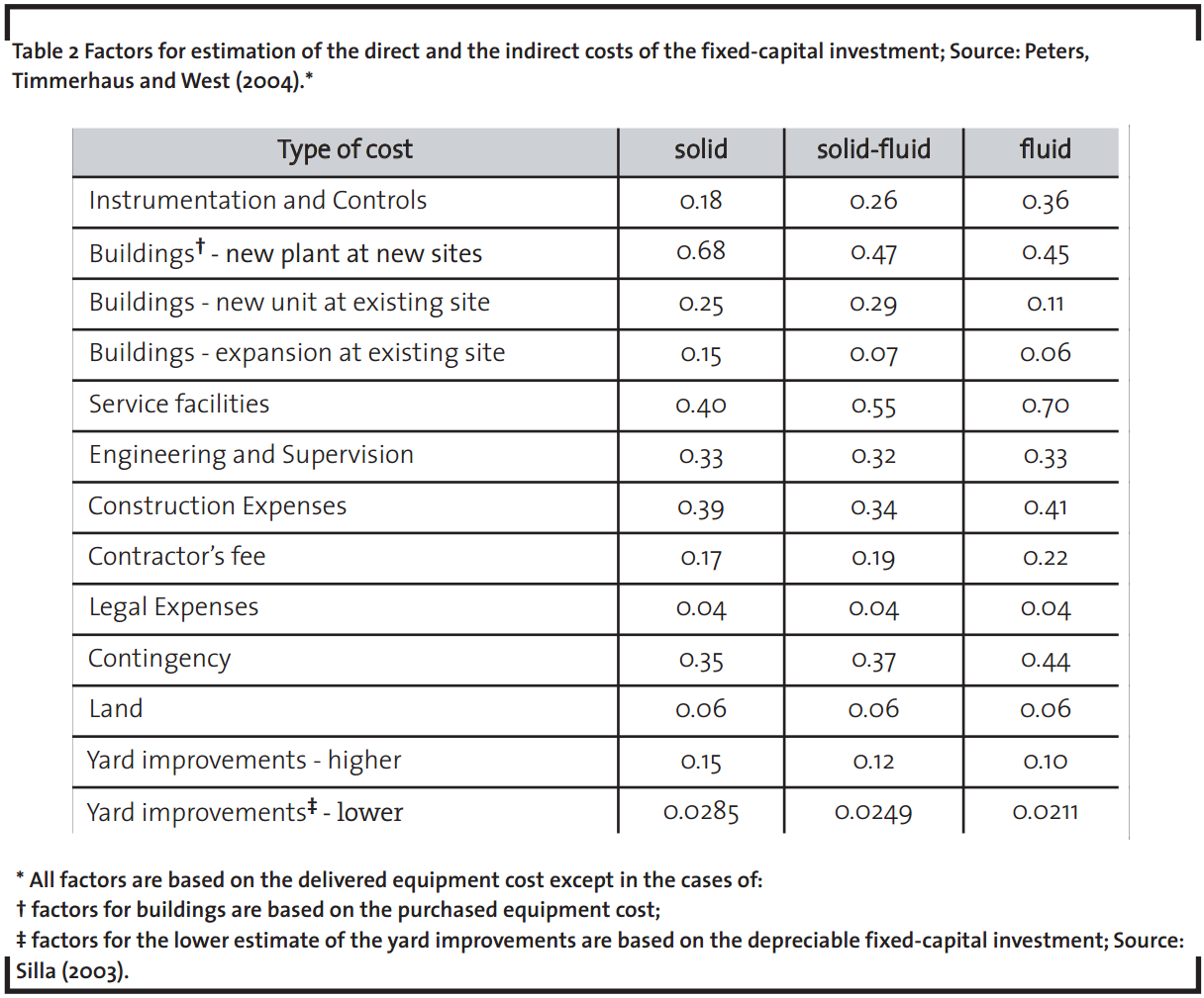
The cost objects within the fixed-capital investment are commonly estimated by multiplication of the purchased or the delivered equipment with a suitable factor. It is important to point out that for many types of costs three different values will be suggested according to the three types of processing plants: solid, solid fluid and fluid processing (see below Table 2; Peters, Timmerhaus and West, 2004). The various types of costs are discussed next.
The instrumentation and controls cost includes the purchased, delivered and the installed cost for any instrumentation and control equipment (such as alarms, sensors, valves, etc.), including all expenses for computer control and supportive software. In the SCENT tool there are two ways of estimating this cost, i.e. a detailed and a rough estimation method.
In the detailed estimation method, instrumentation and controls are considered as separate equipment and estimated based on a dataset including prices for control systems, sensors, alarms and others. The estimation is done in the same way as the estimation of the equipment cost. The source of the database is Woods (2008) and each piece of equipment comes together with individual capacity exponents, installation factors, alloy and additional factors. The purchased cost is linked to the CEPCI cost index and where applicable, exponents are used to correct for scale together with alloy and additional factors.
In the rough estimation method, the factors suggested by Peters, Timmerhaus and West (2004) are used. The corresponding factor, depending on the type of processing plant, is multiplied with the delivered equipment cost, to represent the capital costs related to the instrumentation and controls (Table 2).
The cost object of buildings represents all expenses for process-related buildings (including sub- and superstructures, platforms, stairways), auxiliary buildings (e.g. administration and office, garage, product or spare parts warehouse, safety and security, fire station, shipping office, research and control laboratories), maintenance shops (e.g. electric, piping or machine). This cost includes all necessary building services – plumbing, heating, ventilation, lighting, elevators, telephones, intercommunication systems, painting, fire alarms and others.
The cost of buildings is estimated by multiplying the purchased equipment cost (excluding delivery) with a representative factor. Different values are presented by Peters, Timmerhaus and West (2004) based on three additional considerations: whether a new plant is built at a new site, a new unit is built at an existing site or simply an expansion is made to an existing plant (Table 2). The cost of buildings is lowest in the case of expansion, because most of the required infrastructure already exists and the cost is highest in the case of building new plant at undeveloped site.
The service facilities are all additional process or non-process equipment which are not directly involved in the manufacturing of the end product but are of crucial importance for the whole plant operations. They are commonly referred to as “off-sites” and fall under the category “outside-battery limits”. Brennan (2004) points out that mostly the term “services” is used as synonym for utilities and the term “plant service facilities” also includes buildings.
These include facilities required for the supply of utilities such as steam, water, power, refrigeration, compressed air, and also waste disposal facilities. Other types of facilities which could fall under this cost object are, for example, water treatment and storage, cooling towers, electric substation, air separation plant, fuel storage, waste disposal plant, environmental controls and fire protection. Non-process equipment required for the plant is also estimated as part of this item – office furniture and equipment, shelves, bins, safety and medical equipment, fire extinguishers, hoses and engines, loading stations, and important distribution and packaging equipment – raw material and product storage and handling equipment, blending facilities, etc.
There are three ways of estimating this cost: detailed and rough factorial estimation and through selecting pieces of equipment.
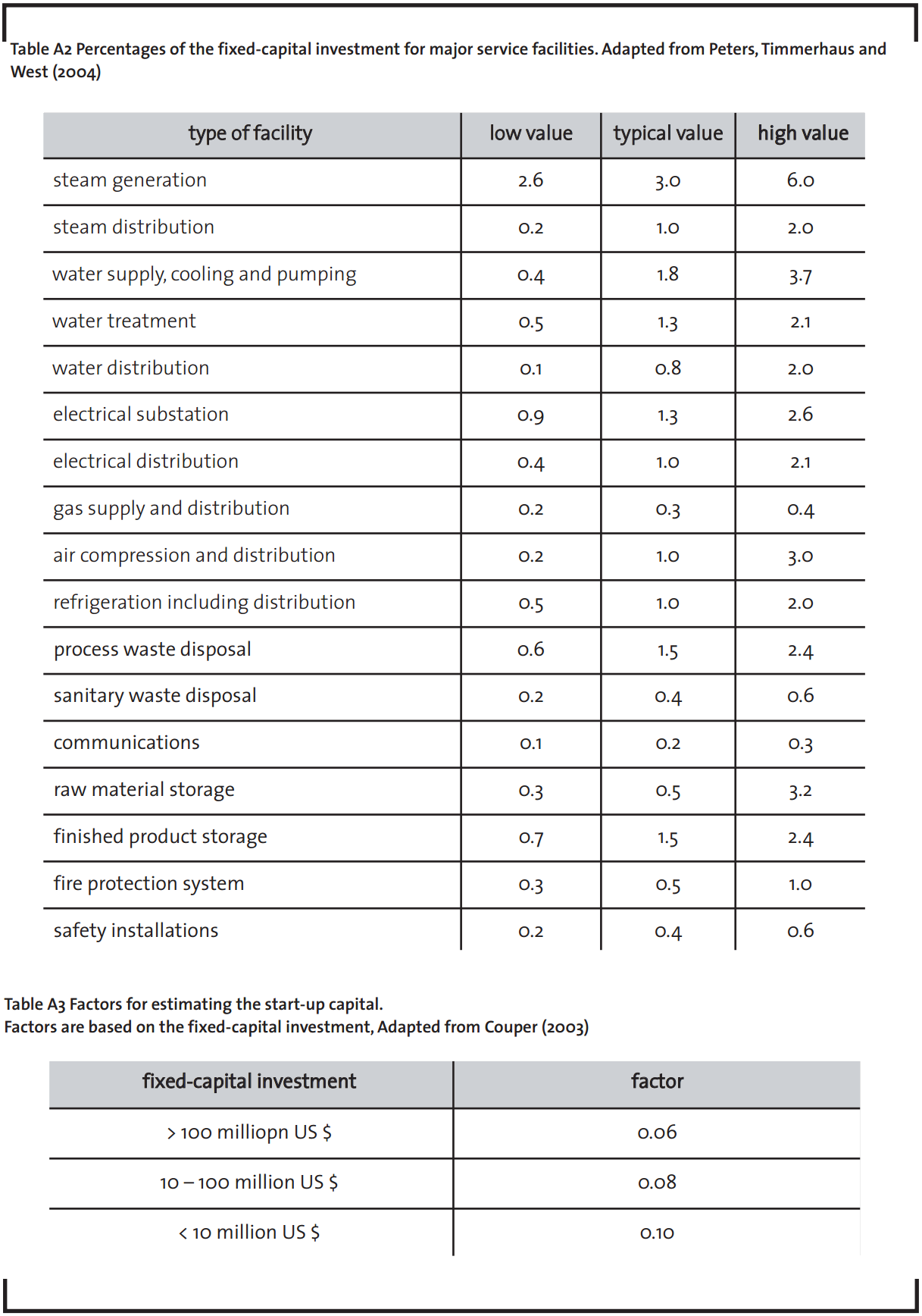
- In the detailed factorial estimation, the estimator is presented with a short list of some of the more common service facilities at manufacturing sites (Appendix Table A1). One can choose between low, typical or high values of percentages of the fixed-capital investment for each of the given facilities.
- The rough factorial estimation method is based on the delivered equipment cost using factors suggested by Peters, Timmerhaus and West (2004) in Table 2.
- As an alternative to the factorial method it is also possible to extract values for the major pieces of equipment required in the service facilities from the cost database (this is possible because Woods (2008) gives cost data for such equipment, e.g. steam turbine or waste water treatment unit).
Engineering and supervision costs include expenses for administration, process design and general engineering, computer graphics, cost engineering, communications; also consultant fees, travel expenses, as well as engineering supervision and inspection.
The category for construction expenses and contractor’s fee comprises all costs for construction, operation, also maintenance of temporary facilities, offices, roads, communications and fencing; all expenses for construction tools and equipment, supervision, accounting, timekeeping and purchasing. Additional costs such as warehouse personnel and expenses, guards, safety, permits, taxes, insurances and interest are estimated as part of this cost object. Peters, Timmerhaus and West suggest separate factors for estimating the contractor’s fee.
In order for the project to be executed, some legal costs are incurred, such as the expenses for the process of identification of applicable federal, state and local regulations, preparation and submission of forms required by regulatory agencies, the process of acquisition of regulatory approval and contract negotiation costs.
When executing new projects, there is high possibility of certain unforeseen events to occur that might cause delays or additional costs. Possible examples are extreme weather conditions (storms, floods), transportation accidents, strikes by transportation or construction personnel, design changes, omissions, errors or inaccuracies in estimation as well as various construction problems. The costs related to such unforeseen events are covered by the contingency capital, which is sometimes also referred to as back-up capital.
It is important to note that compared to other sources (e.g. Couper or Woods) the contingency capital values suggested in Table 2 are on the low side as other sources suggest values around 15–25% of the fixed-capital investment. Therefore, these values are meant for orientation, bearing in mind that for the respective technology studied, different values might be more appropriate. For new technologies the estimator might prefer much higher values, depending on the technology features. It is generally accepted as a rule of thumb that the lower the total value of the project, the higher the contingency capital must be (Table 2).
The land and yard improvements costs include all necessary capital for land surveys and fees, the property cost, and yard improvements such as expenses for site development (site clearing, grading) and landscaping, roads, walkways, railroads, fences, parking areas, etc.
Land and yard improvements are sometimes excluded from the capital investment. Land is considered to be completely recoverable at the end of the plant’s life and therefore does not need to be capitalized. The value for the land cost is suggested to be between 4% and 8% of the delivered equipment cost, with 6% being an adequate average value (Table 2).
The yard improvements are considered to increase the value of the land, so again they do not need to be capitalized (as recoverable) (Silla, 2003). They are estimated using two alternative sets of factors (see Table 2); the first is based on Peters, Timmerhaus and West (2004) and refers to the delivered equipment cost; the second source originates from Silla (2003) and is based on the fixed-capital investment. The first approach (based on the delivered equipment cost) tends to give results that are on the higher side.
Before the plant reaches its regular operational mode it runs through a so-called “start-up” period. During this time, additional expenses will occur such as allowance for testing and adjustment of equipment, piping and others, the calibration of instrumentation and control equipment. The start-up costs include materials, utilities and labour for checking and testing the plant and initial personnel training. These costs are considered part of the capital investment.
There are two approaches for the estimation of this cost: the single- and the multiple-factor approaches both suggested by Couper (2003). The single-factor approach is a percentage of the fixed-capital investment credited to the start-up expenses. The multiple-factor is based on a few items like the number of months for training of the personnel and for the start-up of production, initial inefficiency expenses as percentage of the production costs and others. The multiple-factor approach will not be used in SCENT as it requires data which might not be available for new technologies.
The single-factor approach for estimating the start-up expenses gives three values of percentages (6, 8% and 10%) of the fixed-capital investment depending on the magnitude of the investment. The factor given in Appendix Table A2 is multiplied with the value of the fixed capital investment to determine the start-up estimate.
4.1.4 Working capital
By analogy with the estimation of the startup capital, there are two widely accepted approaches for the estimation of the working capital: the percentage and the inventory method (Couper, 2003). The inventory method takes into consideration few major items: raw materials cost and periods of supply, semifinished and finished products cost, period of sales and others. Such detailed information is likely to be unavailable for a new technology; therefore, the chosen percentage method is presented next.
The percentage method simply estimates the working capital as a percentage of another cost and can be based on either the capital investment or the annual sales. Since for new technologies, there might be a great uncertainty with regard to the sales, the percentage of capital investment was selected as more suitable option. The working capital is between 15% and 30% of the total capital investment. The total capital investment includes two components: the fixed-capital investment and the working capital (see Figure 2). Once the fixed-capital investment is estimated, the working capital is estimated on its basis.
As explained above the working capital is constantly regenerated by income from sales; therefore it strongly depends on the type of sales rate. If a product is sold at relatively constant and uniform yearly rate, then the regeneration of working capital has smaller fluctuations and values between 15% and 25% of the total capital investment are suggested for the working capital. If the product has very high seasonal variations in sales, then higher values are proposed: 20%–30% of the capital investment (Couper, 2003).
4.2 Production cost estimate
As explained above, in SCENT the final production cost estimate is on annual basis. The capital investment cost is annualized to represent the yearly capital recovery expense. The amounts of raw materials required for the manufacturing of the product are estimated based on the material balance. The category “raw materials” consists mostly of chemicals, catalysts and solvents. A database of prices for more than 700 types of chemicals is incorporated in the SCENT tool. The source of these prices is the www.icis.com website (free-of-charge area). These prices were initially published in the 28 August 2006 issue of the Chemical Market Reporter magazine (now existing as ICIS Chemical Business). Most of the prices are from 2006, while some of these prices were recently updated in 2007 and 2008.
The prices in this database are given in US $ and in US customary units (not SI units) – e.g. gal, lb. For this reason – a unit convertor is included in the SCENT tool. For most of the prices, the geographic origin of the price is given and it is very likely that in different areas of the world, the price would be different. For this reason the cost data should be used with caution, the prices in the embedded database serves for orientation and preliminary estimates but wherever possible, more accurate data e.g. from quotations made by possible vendors and suppliers should be used.
The expenses for utilitiessuch as diesel oil, gasoline, natural gas, electricity and water are also estimated from the material and energy balances. A database of prices was compiled mainly from Eurostat and the US Energy Information Administration, with all of the prices being country-specific (the prices are included in the SCENT tool).
The cost data for electricity and natural gas are valid for industrial consumers. Country specific water prices are difficult to obtain. The source used for water prices in SCENT is a 2008 report by NUS Consulting. All of the water prices are unfortunately for household consumers, and some of the countries have country-specific prices, while for the rest – the European average is used. The estimator should note that the prices for household consumers are typically much higher than the local prices for industrial consumers. For preliminary economic estimates, such rough values of water prices are considered acceptable, but they should be replaced by more accurate data when preparing a more detailed estimate.
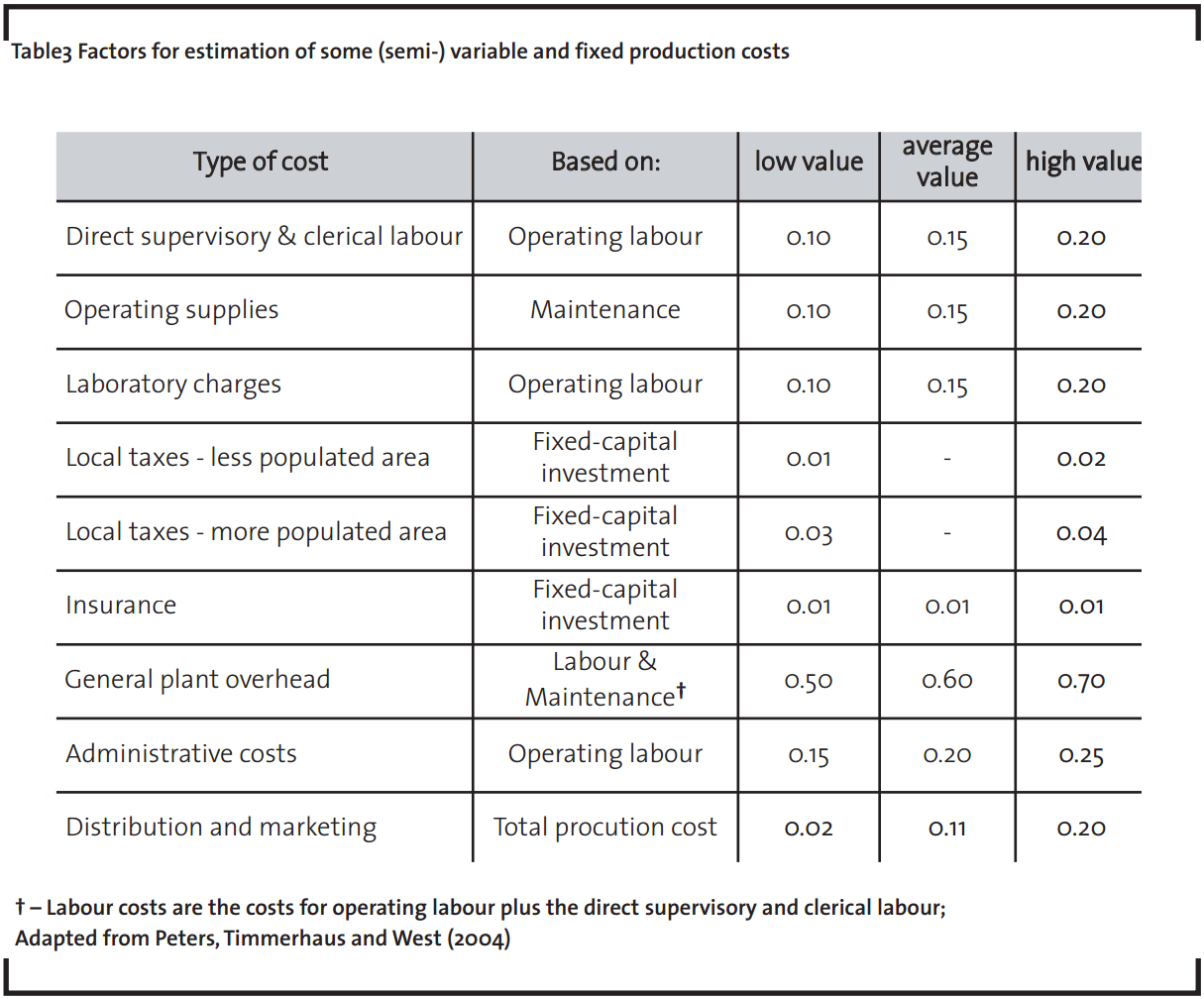
The labour costs are estimated in two parts: operating labour costs and direct supervisory and clerical labour costs. The direct supervisory and clerical labour costs are estimated to be between 10 and 20% of the operating labour costs, with 15% being an average value (Table 3).
The operating labour is estimated by multiplying the number of required employees by the average labour cost in the manufacturing industry in the different countries. The number of required employees could be estimated in three alternative ways:
- Based on the type of equipment. Ulrich (1984) developed a table of the most common types of equipment and assigned a representative number of operators per shift to each type of equipment. For example a heat exchanger requires 0.1 operators per shift and a cooling tower requires 1 operator per shift (the specific values are given in the SCENT tool). This allows estimating the total number of operators required per shift for the plant operations. It is assumed that an employee works 5 shifts of 8 hours per week, for 48 weeks per year. Then, on the base of the load factor of the technology, the required number of full-time employees is estimated.
- Peters, Timmerhaus and West (2004) suggest representative values of required employee-hours for manufacturing 1000 kg of end product. For solid-processing plant, the values are between 4 and 8, for solid-fluid processing plant: between 2 and 4 and for fluid processing plant the suggested values are between 0.33 and 2. On the base of the capacity and the load factor of the technology, the necessary number of employees is estimated.
- Wessel (1952) developed an equation to estimate the labour requirements for production rate of 2000 (short) tons/day (1814 metric tonnes/day). The method gives the number of operator-hours per ton per processing step. A processing step is defined as a step in which a unit operation occurs (Couper, 2003), e.g. filtration or distillation are considered separate steps. Equation (7) below is adapted from Couper (2003):


Y is the operating labour in operator-hours per ton (short ton) per processing step
X is the plant capacity in tons (short tons) per day
B is a constant depending on the type of process: + 0.132 (for batch operations), + 0 (for operations with average labour requirements), – 0.167 (for well-instrumented continuous process).
Once the number of the required employees is estimated through one of the three approaches, this number is multiplied with the country-specific labor cost. The specific salary rates are given in the SCENT tool with the respective sources, namely Eurostat and the US Census Bureau.
The approaches 2 and 3 presented here are based on historical data from the chemical industry and are commonly used as a rule of thumb for preliminary estimates. Ulrich’s approach might be more accurate for new technologies because it is not based on historical data, but on equipment specifics. For this reason it is recommended for new technologies and the other two approaches are simply given as alternatives. As a further argument put forward by Couper (2008) is that Ulrich’s approach is also simpler.
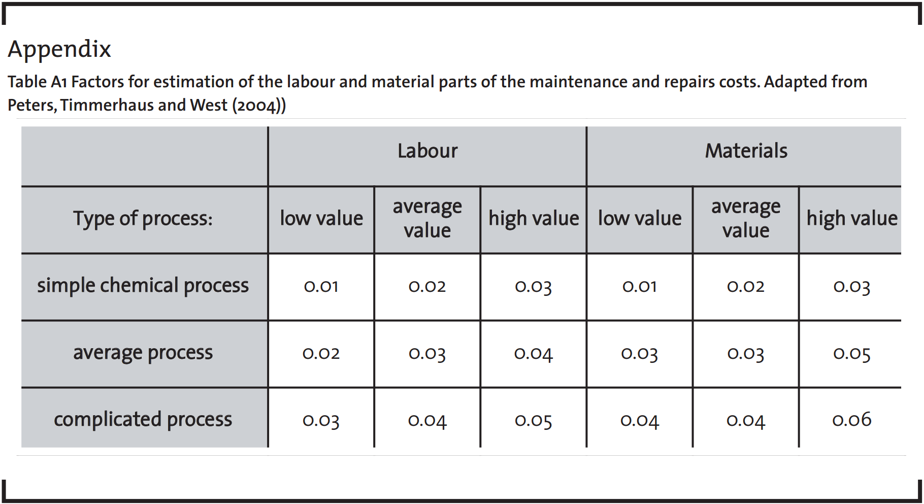
According to Peters, Timmerhaus and West (2004) the maintenance and repairs costs vary depending on the type of chemical process: for a simple chemical process, the maintenance costs are low (2-6%) and tend to rise for an average process (with normal operating conditions: 5-9%) and for a complicated process (or with severe corrosion operating conditions, or with extensive instrumentation: 7-11%). The maintenance and repairs costs refer to the fixed capital investment and have two parts, namely labour and material. The corresponding factors are given in Appendix Table A3 for a low, average and high cost level for each component.
The costs for operating supplies include expenses for lubricants, test chemicals and spare parts and they are estimated at 10 to 20% of the maintenance and repairs costs (Table 3).
Other (semi-) variable costs include the laboratory charges and expenses for patents and royalties. The laboratory charges are estimated at 10 to 20% of the operating labour (Table 3). Another important cost object are the patents and royalties (0 to 6% of the total product cost is suggested by Peters, Timmerhaus and West, 2004). For new or emerging technologies, however, typical percentages might not be correct and that is why this cost might be very specific to the technology in question. For this reason the costs for patents and royalties were excluded from SCENT.
The factors used to estimate the fixed production costs are presented in Table 3 together with the quantity they refer to (second column from the left). Local taxes are likely to differ depending on the location of the plant – and they are estimated at 1-2% of the fixed capital investment in less populated areas and at 3-4% in more populated areas. Insurance is accepted to be roughly 1% of the fixed-capital investment (or less).
The general plant overhead comprises all costs for general plant upkeep, packaging, medical services, safety and protection, storage facilities and others. Important part of this cost is the payroll overhead which is suggested to be typically between 30 and 40% of the labour costs (Couper, 2008). Administrative costs include executive salaries, clerical wages, legal fees, office supplies and communication. These costs are estimated around 15-25% of the operating labour. Distribution and marketing expenses are typically spent on sales offices and salespeople, shipping and advertising (Table 3).
Research and Development costs are excluded from SCENT as for new and/or emerging technologies these might be atypically high and a preliminary estimate might be inaccurate.
The initial capital investment is recovered through depreciation which depends on the discount rate and the lifetime of the manufacturing plant. The applicable depreciation regime is likely to differ by country. Financing (in terms of interest on borrowed capital) must also be included as an annual cost. For new technologies, financing, interest rates, government subsidies, etc. are subject to high uncertainties. For this reason, a strongly simplified method will be used in SCENT. A capital recovery factor αis calculated according to equation (8):

where: α– capital recovery factor (annuity factor), r – interest rate and L – capital recovery period (in years). The annual capital recovery is calculated according to equation (9):

5 Accuracy of the methodology
All factors presented above are based on actual manufacturing plants. It is reported that estimates obtained with them provide uncertainty of the results at ±30% (Couper, 2008). Woods as well as Peters, Timmerhaus and West also suggest the same theoretical accuracy for the cost data provided for the purchased equipment and the factors proposed for estimating the remaining costs.
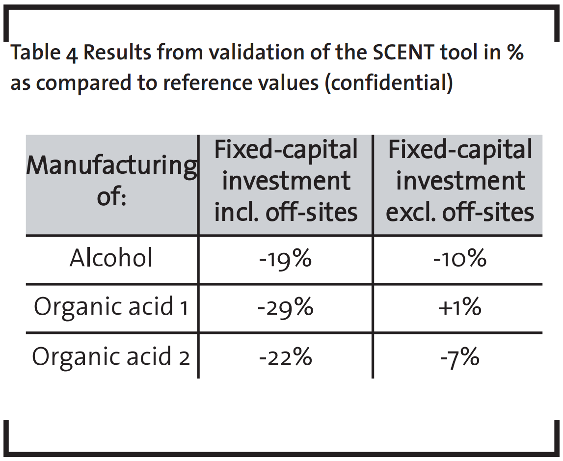
Therefore, it is assumed that the theoretical accuracy of the SCENT tool is also expected to be around ±30%. In order to gain first insight into the accuracy of SCENT, it was validated for three types of manufacturing processes. Due to the confidentiality of the data used, the exact names of the products and overall costs are not presented and only the inaccuracy of this methodology against the cost value reported in the original source is shown.
It was found that the biggest source of inaccuracy is the off-site capital and this is acknowledged as a limitation of this methodology. Therefore the validation was adjusted to exclude the estimation of off-sites and the respective deviations are also given in Table 4.
The main factors affecting the final accuracy are the quality of the input cost data and the accuracy of the factors to estimate the different cost objects. A cost assessment of higher quality can be achieved by investing more resources in obtaining more accurate input prices of equipment as many other cost objects are based on the cost of the purchased equipment. It is important to note that for preliminary purposes, 30% accuracy is quite sufficient and widely accepted in literature (see Couper, 2003 and 2008). A cost assessment of this type is not meant to serve as basis for a final conclusion on the economic viability of a technology. Instead, the ultimate purpose of such preliminary estimate is to formulate a recommendation whether the technology is promising and whether therefore a more accurate estimate using better input data should be prepared, e.g. by application of commercial software tools (see footnote 2) or in close cooperation with equipment suppliers and engineering companies offering turn-key plants.
6 Conclusion and discussion
The methodology presented in this paper and implemented in the SCENT tool offers a comprehensive approach for preparing preliminary economic estimates for plants operated by the process industries. The SCENT tool was developed in the form of a MS Excel file which is simple to use and is publicly available at www.prosuite.org. SCENT focuses particularly on new or emerging technologies for which the available data is typically scarce and/or uncertain.
The methodology uses the factorial approach – cost objects are estimated using factors and percentages on the basis of the purchased equipment cost. The chosen approach is based on an extensive literature survey on methodologies and suitable data. SCENT is operated on a limited amount of data (list of equipment required for the technology). Therefore it is especially practical for new or emerging technologies.
The most important cost item in the estimation process is the purchased and the installed equipment cost, mainly because it is a major part of the fixed-capital investment (can reach up to 80% of it) and also because it is used as a base for the estimation of the remaining cost objects. Against this background, the individual installation, alloy, capacity and additional factors presented by Woods (2008) were used in SCENT since they increase the accuracy of the estimate.
A limitation of the methodology is the fact that all factorial correlations originate from plants and processes based in the USA. Since the process industry is globalized and typical equipment, materials, and design specifications, etc. are similar throughout the world, the selected approach is likely to produce sufficiently accurate preliminary results also for plants operated elsewhere.
While material costs can also be assumed to be globally comparable, there are substantial differences in labour rates, even between countries from the same region. Therefore, a labourrelated installation correction factor is introduced in this paper which accounts for the differences in labour rates among the European Union countries, as well as Norway and the USA. It increases the accuracy of the capital investment estimate.
A database has been compiled with recent prices and costs for nearly 500 pieces of equipment, selected utilities, over 700 types of chemicals and the labour costs in most European
countries.
This database also includes a short list of typical environmental protection expenses. It is acknowledged in this paper that this list is not representative and insufficient to estimate all environmental protection expenses which might occur for a technology.
More data would be required in order to reflect more accurately the differences between the countries: country-specific costs for environmental protection expenses or taxes, infrastructure and transportation-related costs (currently delivery charges are assumed to be fixed at 10% of the purchased equipment cost, despite location), regulations, local laws, labour productivity and others.
In effort to develop a standardized approach, few cost items were deliberately excluded from the analysis because they might vary substantially for new or emerging technologies: costs for research and development, patents and royalties, subsidies or interest rates. Possible technological learning with time is also neglected. Technological learning can, however, be incorporated in SCENT when estimating the capital investment. If projects which are similar to the emerging technology have already been executed, one can review the different cost objects and conclude whether some of them showed substantially higher or lower final costs as compared to initially estimated. The methodology also allows for accounting for expected higher yields and the improvement of any other parameter, but this is again technology-specific and cannot be included in a standardized approach.
This methodology is hence capable of offering reliable estimates for preliminary purposes. This was confirmed by applying the SCENTtool for three types of manufacturing processes. The resulting estimates of the fixed-capital investment were within the expected accuracy range, with the highest in accuracy observed for the off-site capital. This is acknowledged as a limitation of this methodology. Based on the validation runs, the literature information on the method and the quality of the data used, we conclude that the results generated with the SCENT tool have a theoretical uncertainty of ±30%.
In conclusion, SCENT is recommended as suitable approach to estimate the production costs of new or emerging technologies.
References
Blok, K. (2008): Introduction to Energy Analysis, Techne Press, Washington D.C.
Brennan, D.J. (2004): Process Industry Economics: An International Perspective, IChemE, London.
Couper, J.R. (2003): Process Engineering Economics., Marcel Dekker, New York.
Couper, J.R. (2008): Process Economics section, in: Green, D.W., Perry, R.H., (Eds.) Perry’s Chemical Engineering Handbook, 8th ed., McGraw-Hill, Columbus (OH).
Dysert, L.R. (2003):. Sharpen Your Cost Estimating Skills, Cost Engineering, 45(6), 22-30.
Economy Watch (2010): retrieved 6-Sep-2010, http://www.economywatch.com/worldindustries/capital-intensive.html.
Guthrie, K.M. (1969), Chemical Engineering, 114–156.
Guthrie, K.M. (1974): Process Plant Estimating, Evaluation and Control, Craftman Book Company of America, Solana Beach, CA.
Hand, W.E. (1958): Petroleum Refiner. September 1958: 331–334.
Holland, F.A., Wilkinson, J.K. (1997): Process Economics section, Perry’s Chemical Engineering Handbook, 7th ed., McGraw-Hill, Columbus (OH):.
Peters, M.S., Timmerhaus, K., West, R. (2002): Plant Design and Economics for Chemical Engineers; McGraw-Hill, Columbus (OH).
Silla, H. (2003): Chemical Process Engineering (Design and Economics), Marcel Dekker, New York.
Towler, G., Sinnott, R.K. (2007): Chemical Engineering Design: Principles, Practice and Economics of Plant and Process Design, Butterworth-Heinemann, Oxford.
Ulrich, G.D. (1984): A Guide to Chemical Engineering Process Design and Economics, John Wiley & Sons Inc, Hoboken, NJ.
Wells, G.L., Rose, L.M. (1986): The art of chemical process design, Elsevier Science Pub, Amsterdam.
Woods, D.R.(2008): Rules of Thumb in Engineering Practice, Wiley-VCH, Hoboken, NJ.
Wroth, W.F. (1960.): Chemical Engineering, 1960:204.
Appendix